Dimensions, Segmentation and
Multiscale Time Series
Rafal Baranowski
Department of Statistics
London School of Economics and Political Sciences
This dissertation is submitted for the degree of
Doctor of Philosophy
I certify that the thesis I have presented for examination for the PhD degree of the London School of Economics and Political Science is solely my own work other than where I have clearly indicated that it is the work of others (in which case the extent of any work carried out jointly by me and any other person is clearly identified in it). The copyright of this thesis rests with the author. Quotation from it is permitted, provided that full acknowledgement is made. This thesis may not be reproduced without my prior written consent. I warrant that this authorisation does not, to the best of my belief, infringe the rights of any third party. I declare that my thesis consists of about 65000 words.
I confirm that Chapter4was jointly co-authored with Doctor Yining Chen and Professor Piotr Fryzlewicz and I contributed 60% of this work.
I confirm that Chapter 5was jointly co-authored with Professor Piotr Fryzlewicz and I contributed 80% of this work.
Chapters3 and 4have been submitted to peer-reviewed statistical journals. We plan to submit Chapter 5for publication soon.
First and foremost, I would like to thank my supervisor, Professor Piotr Fryzlewicz, for his constant guidance, enthusiasm, encouragement and extremely professional feedback on my work. I am also grateful to Doctor Yining Chen, with whom I had the luck to work on a research paper which constitutes one of the chapters in this thesis.
I wish to express my gratitude to all the staff and students in the Department of Statistics at the London School of Economics for providing me with a great working environment. I am also deeply grateful for the financial support of the London School of Economics Research Studentship without which this thesis could not have been neither undertaken nor completed.
In this dissertation, we study the following three statistical problems.
First, we consider a high-dimensional data framework, where the number of covariates potentially affecting the response is large relatively to the sample size. In this setting, some of the covariates are observed to exhibit an impact on the response spuriously. Addressing this issue, we rank the covariates according to their impact on the response and use certain subsampling scheme to identify the covariates which non-spuriously appear at the top of the ranking. We study the conditions under which such set is unique and show that, with high probability, it can be recovered from the data by our procedure, for rankings based on measures commonly used in statistics. We illustrate its good practical performance in an extensive comparative simulation study and on microarray data.
and the UK House Price Index
Finally, we introduce a class of univariate multiscale time series models and propose an estimation procedure to fit those models from the data. We demonstrate that our proposal, with a large probability, correctly identifies important timescales, under the framework in which the largest timescale in the model diverges with the sample size. A good empirical performance of the method is illustrated in an application to high-frequency financial returns for stocks listed on New York Stock Exchange.
List of figures 13
List of tables 14
List of algorithms 17
1 Introduction 18
2 Literature review 22
2.1 High-dimensional variable selection . . . 22
2.1.1 Variable selection via Penalised Likelihood minimisation . . . 25
2.1.1.1 PLH withℓ0-norm type penalty . . . 26
2.1.1.2 PLH withℓ1-norm and ℓ2-norm type penalties . . . 26
2.1.1.3 PLH with other types of penalties . . . 28
2.1.2 Variable screening methods . . . 28
2.1.3 Subsampling in variable selection . . . 30
2.2 Data segmentation and multiple change-point detection . . . 31
2.2.1 Canonical change-point detection problem . . . 33
2.2.1.1 Multivariate optimisation . . . 33
2.2.1.2 Binary Segmentation . . . 34
2.2.2 Regression change-point models . . . 39
2.2.2.1 Methodology ofBai and Perron (1998) . . . 40
2.2.2.2 Trend filtering . . . 41
2.2.3 Other change-point detection problems . . . 42
2.2.3.1 Change in variance and/or mean . . . 42
2.2.3.2 Nonparametric change-point detection . . . 43
2.3 Multiscale time series models . . . 44
2.3.1 Multiscale time series models of Ferreira et al. (2006) . . . 45
2.3.2 Mixed Data Sampling Regression Models . . . 45
3 Ranking-Based Variable Selection 47 3.1 Introduction . . . 47
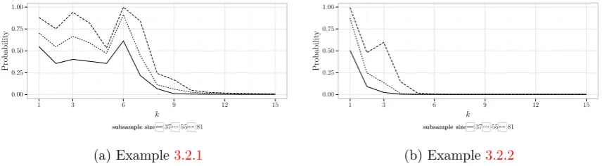
3.2 Motivating examples . . . 52
3.3 Methodology of Ranking-Based Variable Selection . . . 54
3.3.1 Notation . . . 54
3.3.2 Definition of a k-top-ranked and the top-ranked set . . . 54
3.3.3 Top-ranked set for a class of variable rankings . . . 55
3.3.4 Ranking-Based Variable Selection . . . 58
3.3.5 The Ranking-Based Variable Selection algorithm . . . 60
3.3.6 Relations to existing methodology . . . 61
3.3.6.1 Stability selection . . . 61
3.3.6.2 The bootstrapped rankings ofHall and Miller (2009a) . 61 3.3.6.3 Computational complexity of the related methods . . . . 62
3.4 Theoretical results . . . 63
3.5 Iterative extension of RBVS . . . 65
3.6 Simulation study . . . 66
3.6.2 Choice of parameters of the RBVS algorithm . . . 68
3.6.3 Simulation models . . . 69
3.6.4 Comments on the results . . . 70
3.7 Data examples . . . 78
3.7.1 Prostate cancer data set . . . 78
3.7.2 Boston housing data set . . . 80
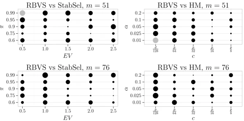
3.8 High-dimensional simulation study . . . 82
3.9 Computational aspects . . . 98
3.9.1 Details of the implementation of the RBVS algorithm . . . 98
3.9.2 Algorithmic differences between RBVS and StabSel . . . 99
3.9.3 Simulation code . . . 101
3.10 Proofs . . . 104
3.10.1 Proof of Proposition 3.3.1 . . . 104
3.10.2 Proof of Theorem 3.4.1 and discussion of some of its aspects. . . . 106
4 Narrowest-Over-Threshold change-point detection 112 4.1 Introduction . . . 112
4.2 Methodology . . . 119
4.2.1 Setup . . . 119
4.2.2 Main idea . . . 121
4.2.3 Log-likelihood ratios and contrast functions . . . 123
4.2.3.1 Scenario (S1) . . . 123
4.2.3.2 Scenario (S2) . . . 125
4.2.3.3 Scenario (S3) . . . 126
4.2.3.4 Scenario (S4) . . . 127
4.2.4 The NOT algorithm . . . 128
4.3 Computational aspects . . . 131
4.3.1 Computing contrast functions in linear time . . . 131
4.3.2 The NOT solution path algorithm . . . 132
4.3.3 An illustrative example . . . 135
4.3.4 Parameter choice . . . 136
4.3.4.1 Choice ofM . . . 136
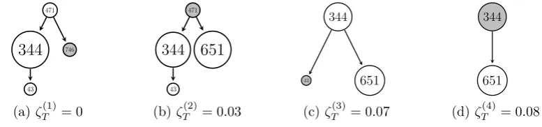
4.3.4.2 Choice of the thresholdζT . . . 137
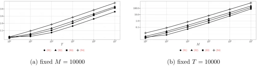
4.3.5 Computational complexity of the NOT and NOT solution path algorithms . . . 138
4.4 Simulation study . . . 140
4.4.1 Simulation methods . . . 140
4.4.2 Simulation models . . . 143
4.4.3 Results and discussion . . . 150
4.5 Real data analysis . . . 153
4.5.1 OPEC Reference Basket oil price . . . 153
4.5.2 Temperature anomalies . . . 156
4.5.3 UK House Price Index . . . 157
4.6 Proofs . . . 160
4.6.1 Some useful lemmas . . . 160
4.6.1.1 The piecewise constant case . . . 160
4.6.1.2 The piecewise linear continuous case . . . 163
4.6.2 Proof of Theorem 4.2.1 . . . 167
4.6.3 Proof of Theorem 4.2.2 . . . 175
5 Multiscale autoregression 180 5.1 Introduction . . . 180
5.2.1 Notation . . . 184
5.2.2 Large deviations for the OLS estimator in AR(p) . . . 185
5.2.3 Estimation of the timescales with NOT . . . 186
5.2.4 AMAR algorithm and its theoretical properties. . . 188
5.3 Practicalities and simulated examples . . . 191
5.3.1 Parameter choice and other practicalities . . . 191
5.3.1.1 Choice of the thresholdζT . . . 191
5.3.1.2 Choice ofp . . . 192
5.3.1.3 Choice ofM . . . 192
5.3.1.4 Computational complexity. . . 192
5.3.2 Simulation study . . . 193
5.4 Application to high-frequency data from NYSE TAQ database . . . 196
5.4.1 Data preprocessing . . . 197
5.4.2 Rolling window analysis . . . 198
5.4.3 Results and discussion . . . 200
5.4.4 Simulated data with real volatility . . . 205
5.5 Large deviations for LSE estimators in stationary AR(p) models . . . 206
5.5.1 Some properties of the B matrix . . . 207
5.5.2 Two useful lemmas . . . 209
5.5.3 Proof of Theorem 5.2.1 . . . 210
5.6 Proof of Theorem 5.2.2 . . . 216
6 Conclusions 223
3.1 Probabilities corresponding to the most frequently occurring subsets of
covariates in Example 3.2.1 and 3.2.2. . . 53
3.2 Classification rates in the application to the prostate cancer data set. . . 79
3.3 Probabilities corresponding to the most frequently occurring subsets of covariates in the application to the Boston housing data set. . . 80
4.1 Motivating example . . . 118
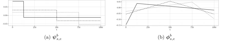
4.2 Examples of ϕbs,e and ψbs,e . . . 124
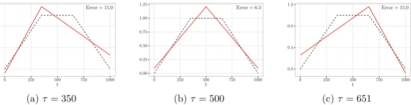
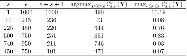
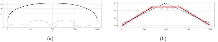
4.3 Illustrative example . . . 136
4.4 Segmentation trees obtained with Algorithm 4.7 . . . 137
4.5 Execution times of Algorithm4.7 . . . 140
4.6 Examples of data generated from simulation models studied in Section 4.4.2.144 4.7 Change-point analysis on the daily OPEC Reference Basket oil price . . . 154
4.8 Change-point analysis for the GISSTEMP data set . . . 156
4.9 Change-point analysis for the monthly percentage changes in the UK House Price Index . . . 158
5.1 Example of high-frequency trades data for Apple Inc. . . 183
3.1 Computational complexity of Algorithm 3.3 and its competitors . . . 63
3.2 Simulation results for Model (A) . . . 73
3.3 Simulation results for Model (B) . . . 74
3.4 Simulation results for Model (C) . . . 75
3.5 Simulation results for Model (D). . . 76
3.6 Simulation results for Model (E) . . . 77
3.7 Prediction errors in the Boston housing data example . . . 82
3.8 Simulation results in the high-dimensional example form = 50, s= 5 and K = 0 . . . 84
3.9 Simulation results in the high-dimensional example for m = 100, s = 5 and K = 0 . . . 85
3.10 Simulation results in the high-dimensional example for m = n2, s= 5 and K = 0 . . . 86
3.11 Simulation results in the high-dimensional example form = 50, s= 5 and K = 5 . . . 87
3.12 Simulation results in the high-dimensional example for m = 100, s = 5 and K = 5 . . . 88
3.14 Simulation results in the high-dimensional example for m = 50, s = 10
and K = 0 . . . 90
3.15 Simulation results in the high-dimensional example for m = 100,s= 10 and K = 0 . . . 91
3.16 Simulation results in the high-dimensional example form= n2,s = 10 and K = 0 . . . 92
3.17 Simulation results in the high-dimensional example for m = 50, s = 10 and K = 5 . . . 93
3.18 Simulation results in the high-dimensional example for m = 100,s= 10 and K = 5 . . . 94
3.19 Simulation results in the high-dimensional example form= n2,s = 10 and K = 5 . . . 95
3.20 Computation times in the high-dimensional example for s= 5 andK = 0 96 3.21 Informal comparison of the RBVS and StabSel algorithms . . . 100
4.1 Intervals considered in Figure 4.3a. . . 135
4.2 Simularation results for εt∼ N(0,1) . . . 146
4.3 Simularation results for εt∼ N(0,2) . . . 147
4.4 Simularation results for εt∼Laplace 0,(√2)−1 . . . 148
4.5 Simularation results for εt∼(3/5)1/2t5 . . . 149
4.6 Change-points dected in the log-returns of the daily oil price series . . . . 154
5.1 Simulation results for the data following (5.1) with parameters given in Section 5.3.2 . . . 195
5.4 Out-of sample performance of the forecasts obtained with AMAR for 5-minute returns with p= 960 . . . 202
5.5 Out-of sample performance of the forecasts obtained with AMAR for 10-minute returns with p= 240 . . . 203
5.6 Out-of sample performance of the forecasts obtained with AMAR for 10-minute returns with p= 480 . . . 204
2.1 Binary Segmentation . . . 35
2.2 Wild Binary Segmentation . . . 37
3.3 Ranking-Based Variable Selection . . . 60
3.4 Iterative Ranking-Based Variable Selection . . . 66
3.5 Top-ranked sets . . . 99
4.6 Narrowest-Over-Threshold algorithm . . . 128
4.7 NOT solution path . . . 133
5.8 NOT algorithm for estimation of the time-scales in AMAR models . . . . 187
5.9 AMAR algorithm . . . 188
Introduction
Many questions that arise in modern statistics are inspired by high-dimensional data sets, that are nowadays ubiquitous in fields such as genomics, neuroscience, high-frequency finance or economics, to name but a few. For example, a substantial progress has been made over past 20 years in the high-dimensional regression which is now an essential tool in genomics (Bühlmann et al.,2014).
The core chapters of this thesis propose methodologies to tackle three statistical prob-lems: variable selection in high-dimensional data, change-point detection, segmentation and nonparametric function estimation and multiscale modelling of univariate time series. In Chapter 2, we review the statical literature relevant to these problems. Each of the subsequent three chapters begin with an introductory section, where we give further motivations for our work. The remainder is structured as follows.
Chapter 3. Ranking-Based Variable Selection for high-dimensional data
and show that it can be successfully recovered from the data by our procedure. Unlike the majority of the existing high-dimensional variable selection techniques, RBVS does not depend on any thresholding or regularity parameters. Moreover, RBVS does not require any model restrictions on the relationship between the response and covariates, it is therefore widely applicable, both in a parametric and non-parametric context. We illustrate its good practical performance in an extensive comparative simulation study and on real data. The RBVS algorithm is implemented in the publicly available R packages rbvs (Baranowski et al., 2015)
and rbvsGPU Baranowski (2016).
Chapter 4. Narrowest-Over-Threshold detection of multiple change-points
and change-point-like features
NOT in detecting the number and locations of generalised change-points, and discuss how to extend the proof to other settings. The NOT estimators are easy to implement and rapid to compute: the entire threshold-indexed solution path can be computed in close-to-linear time. Importantly, the NOT approach is easy to extend by the user to tailor to their own needs. There is no single competitor, but we show that the performance of NOT matches or surpasses the state of the art in the scenarios tested. Our methodology is implemented in the R package
not (Baranowski et al., 2016b).
Chapter 5. Multiscale autoregression on adaptively detected timescales
Motivated by the notoriously difficult task of predicting high-frequency financial returns, in Chapter 5we introduce Adaptive Multiscale Autoregressive (AMAR) time series models, where the quantity of interest is explicitly modeled as linearly dependent on its own past averages over unknown timescales. Combining the Ordinary Least Square method with the Narrowest-Over-Threshold approach described in Chapter 4, we propose an estimation procedure for identifying both the number and locations of the relevant timescales from the data. We demonstrate that this procedure consistently recovers the timescales under the framework in which both the number of the timescales and the largest timescale diverge with the sample size. In an application to data from the New York Stock Exchange Trades and Quotes Database, we show that our proposal offers relatively good performance in terms of the out-of-sample forecasting of high-frequency financial returns. The proposed methodology is implemented in the R package amar (Baranowski and
Fryzlewicz, 2016a).
Chapter 6 summarises our contributions and points a number of directions for future
research.
from each other, as they are inspired by differently structured data. However, from the methodological and theoretical point of view, there is a common ground between those chapters, namely high-dimensionality. This is due to the fact that the complexity of the considered problems, measured either in terms of the number of covariates (Chapter 3) or in terms of the number of parameters in the corresponding models (Chapters4 and
Literature review
In this chapter, we provide a review of the statistical literature related to the problems covered in this thesis: high-dimensional variable selection, multiple change-point detection and multiscale time series modelling.
2.1
High-dimensional variable selection
Suppose we observe Y1, . . . , Yn, being n observations of the response, and that for each i = 1, . . . , n there are p predictors Xi1, . . . , Xip which potentially influence Y. In this
thesis, the variable selection problem is understood as the situation in which only a small number of predictorsS ⊂ {1, . . . , p}contribute to the response and our aim is to use the observed sample to identify those. When plarge in comparison to the sample size n, the
variable selection problem is said to be high-dimensional.
machine learning (Du Jardin,2010;Rakotomamonjy, 2003), to name a few. An extensive list of high-dimensional data analysis problems can be found in Donoho (2000) and
Bühlmann et al. (2016). There exists a large body of statistical literature proposing methodologies designed to tackle high-dimensional data, an excellent overview of which can be found in Fan and Lv (2010), Bühlmann et al.(2011), Hastie et al.(2015) and
Bühlmann et al. (2016). In this section, we briefly discuss different approaches to the high-dimensional variable selection problem, knowledge of which is vital in Chapter 3, where we propose our contribution to the problem.
On a broad level, we group the existing variable selection techniques according to the assumptions on the relationship between the response and the predictors, distinguishing three scenarios. The vast majority of the literature on the variable selection problem studies the following Linear Regression Model (LRM)
Yi =β0+ p
X
j=1
βjXij+εi, , i= 1, . . . , n (2.1)
where β0, β1, . . . , βp ∈ R are the unknown regression coefficients and εi is the random
error term, typically required to satisfy Eεi = 0, Eε2i =σ2 and Eεiεj ̸= 0 for i̸= j. The
set of the variables that contribute to Y is then simply defined as
S ={1≤j ≤p:βj ̸= 0}. (2.2)
Let EYi|(Xi1, . . . , Xip) denote the conditional expectation of Y given Xi1, . . . , Xip.
Hereafter we assume that E|Yi|< ∞, which ensures that the conditional expectation
Generalised Linear Models (McCullagh and Nelder, 1989, GLMs) of the form
EYi|(Xi1, . . . , Xip) =g−1( p
X
j=1
β0+βjXij), (2.3)
where β0, β1, . . . , βp ∈R are again unknown regression coefficients and g :R7→R is the
(invertible) link function. In (2.3) the set of important variables is defined as (2.2). Finally, the third scenario with respect to which we discuss the variable selection techniques is the nonparametric regression model, where
EYi|(Xi1, . . . , Xip) =f(Xi1, . . . , Xip), (2.4)
for an unknown, measurable function f : Rp 7→ R. Here the important variables are defined as
S ={1≤j ≤p: EYi|(Xi1, . . . , Xip) functionally depends on Xij}. (2.5)
Regardless of the nature of the relationship between the response and the predictors, it is commonly assumed that the number of variables inS is small in comparison to p.
In the context of LRM and GLMs, this condition is known as thesparsity assumption. In the remainder of this section, we assume that β0 = 0 in (2.1) and (2.3) and
denote byZi = (Yi, Xi1, . . . , Xip)′ and β = (β1, . . . , βp)′. For any q ≥1, the ℓq-norm of
any vector v∈ Rn is defined as ∥v∥ q =
Pn
j=1|vj|q
1/q
. Additionally, for q = 0 we set ∥v∥0 =Pn
j=1I(vi ̸= 0), i.e. the number of non-zero coordinates of v. Although ∥v∥0 is
not a properly defined norm, as it does not satisfy the absolute scalability condition, we refer to∥v∥0 as the ℓ0-norm of v, which is a common practice in the variable selection
2.1.1
Variable selection via Penalised Likelihood minimisation
A substantial number of the variable selection techniques proposed in the context of (2.1) or (2.3), are derived from the solution of the following Penalised Likelihood (PLH)
minimisation problem
argminβ∈Rp(−2ℓ(β|Z1, . . . ,Zn) + penλ(β)), (2.6) whereℓ(β|Z1, . . . ,Zn) is the log-likelihood of βgiven Z1, . . . ,Zn and penλ is the penalty
function depending on the tuning parameters vector λ= (λ0, . . . , λK) for some integer K ≥ 0. Heuristically speaking, the aim of (2.6) is to find the estimates of β which guarantee that the resulting model fits the data well, but also satisfies some additional constrains on its complexity. Let ˆβ=βˆ1, . . . ,βˆp
denote a solution of (2.6). Typically, the penalty function is designed such that (for an appropriately chosenλ) a large number of ˆβj’s are shrunk to zero. The resulting estimate of S is then defined as
ˆ
S ={1≤j ≤p: ˆβj ̸= 0}. (2.7)
One of the most widely-studied examples of PLH is derived from the linear model (2.1) with the standard Gaussian i.i.d. noise. After omitting constants which does not change the minimum, (2.6) in the Guassian linear model simplifies to
argminβ∈Rp
n
X
i=1
Yi−
p
X
j=1 βjXij
2
+ penλ(β)
2.1.1.1 PLH with ℓ0-norm type penalty
Many classic model selection tools can be formulated as the PLH minimisation problem with the penalty function of the following form
penλ(β) =λ0∥β∥0, (2.9)
where λ1 >0. For example, setting λ0 = 2 recovers the Akaike’s information criterion
(Akaike, 1998); λ0 = log(n) yields the Schwarz’s information criterion (Schwarz, 1978).
Some works propose modifications of the classic information criteria addressing probles arrising in the high-dimensional variable selection, see e.g. Bogdan et al. (2004) or Chen and Chen(2008). However, from the computational point of view, solving (2.6) with the penalty given by (2.9) requires an exhaustive search over all subsets of {1, . . . , p}, hence it is not feasible ifp is larger than a few dozens (Candes and Tao,2007).
2.1.1.2 PLH with ℓ1-norm and ℓ2-norm type penalties
A popular class of penalties, which yield computationally tractable PLHs is of the form
penλ(β) = p
X
j=1
λj|βj|, (2.10)
where λj >0 for all j = 1, . . . , p. When λj ≡λ0 for someλ0 >0, (2.10) simplifies to
penλ(β) =λ0∥β∥1, (2.11)
which recovers the penalty introduced by Alliney and Ruzinsky (1994) andTibshirani
coefficients shrunk to be exactly zero. Lokhorst (1999); Park and Hastie (2007); Shevade and Keerthi(2003);Van de Geer (2008) study variable selection with the (2.11) penalty in the GLMs, for a disscusion of these and other developements of the Lasso methodology, seeTibshirani (2011) and Bühlmann et al.(2011).
Zou and Hastie (2005) observe that, in the situation when two or more important predictors are highly correlated, Lasso tends to select only one of them. In order to deal with this issue,Zou and Hastie (2005) consider the elastic net penalty of the following form
penλ(β) = λ0∥β∥1+λ1∥β∥ 2
2, (2.12)
with λ0, λ1 ≥0. When λ0 = 0, (2.12) simplifies to the classic ridge penalty (Hoerl and Kennard, 1970).
Variants of (2.10) withλj possibly different for eachj = 1, . . . , p, have been also
exten-sively studied in the literature. For example,Zou(2006) suggests to set λj =λ0
βˆ
OLS j
−γ
, where ˆβjOLS denotes the simple OLS estimate of βj and γ > 0 is a tuning parameter,
and shows that this approach yields certain optimality properties. Meinshausen and Bühlmann (2010) suggest to set the penalty parameters to λj = λ0Uj−1, where Uj’s
are independently drawn from the uniform distribution. This, combined with their subsampling scheme discussed in Section3.3.6, yields a method that successfully recovers
S in certain settings in which the standard Lasso fails. Another interesting development can be found inBogdan et al. (2015), who propose the SLOPE penalty defined as
penλ(β) = p
X
j=1
λj|βj:p|,
under orthogonal designs, SLOPE allows for variable selection with a control of the False Discovery Rate (Benjamini and Hochberg, 1995, FDR); Su et al. (2016) demonstrate that the SLOPE estimates ofβ achieve minimax rates in theℓ2-norm sense.
2.1.1.3 PLH with other types of penalties
Fan and Li(2001) propose yet another class of penalty functions, which are designed to return asymptotically unbiased, sparse and continuous in the data estimates of β. They note that ℓq-based penalties in general do not satisfy some of those requirements and
consider
penλ(β) = p
X
j=1
pλ(|βj|), (2.13)
where pλ is defined fort ≥0 through the derivative
p′λ(t) =λ0 I(t≤λ0) + max
{aλ0−t,0}
(a−1)λ0 I
(t > λ0)
!
,
and a >2 is a tuning parameter. Fan and Li (2001) prove that the solutions of (2.8)
with the penalty function specified this way satisfies all aforementioned requirements.
Zhang (2010) considers the penalty of form given by (2.13) with
pλ(t) =λ0
Z t
0 max
{1−x/(λ0γ),0}dx (2.14)
for someγ >0. PLH estimates with this penalty are asymptotically unbiased and attain
certain minimax convergence rates for the estimation of β.
2.1.2
Variable screening methods
minimisation of PLH. First, theoretical conditions required for the consistency of the estimates given by (2.6) are unlikely to be satisfied when p is large in relation to n.
Second, solving (2.6) for large values of p and n is typically computationally expensive.
To tackle those issues in the context of (2.1),Fan and Lv (2008) introduce the concept of
variable screening, defined as follows. Let ˆωj be a measure evaluating the impact of the j’th predictor Xij on the responseYi (e.g. Pearson correlation coefficient), calculated for
the sampleZ1, . . . , Zn and let dn < p be an integer, preferably smaller than n. Variable
screening is then simply defined as the act of removing predictors which exhibit week relationship to the response. Denote by
ˆ
Sdn ={1≤j ≤p: ˆωj is among the first dn largest of all}, (2.15)
i.e. the set of variables that survive after the screening. The variable screening based on the measure ˆωj is said to possesthe sure screening property if
P
S ⊂Sˆdn
→
n 1. (2.16)
Fan and Lv (2008) show that in the linear model (2.1), the variable screening based on the Pearson correlation coefficient, termed as Sure Independence Screening (SIS), achieves the sure screening property, under certain restrictions on the correlation between predictors. If this is satisfied for dn comparable to the sample size n, we can expect
better estimation accuracy by applying the PLH estimation directly on the reduced set of predictors ˆSdn. Importantly, the sample correlations are quick to compute, therefore SIS provides a solution to the aforementioned problems in (2.1).
τ correlation (Li et al., 2012a) or distance correlation (Li et al., 2012b). An excellent
overview of these developments can be found inLiu et al. (2015).
2.1.3
Subsampling in variable selection
A particular difficulty in performing variable selection or variable screening in high-dimensional data using techniques described in the previous sections, is that their performance is sensitive to the choice of the tuning parameters parameters (Fan and Tang, 2013; Meinshausen and Bühlmann, 2010). A variant of cross-validation (CV), so called k-fold CV, where 1 ≤ k ≤ n, is one of the most popular methods employed
to choose the tuning parameters (Arlot et al., 2010; Friedman et al., 2001). In this method, the original sample is randomly divided into k subsamples of approximately
equal length. Next, each subsample is used as the validation set, on which a number of models, corresponding to different tuning parameters and fitted on the remaining data, are evaluated and the parameter yielding the best model in terms of the average evaluation criterion is selected. Typically, k-fold CV is used in conjunction with a
criterion that asses the predictive power of the model, e.g. the Mean Squared Error in LRM.
2.2
Data segmentation and multiple change-point
detection
Let Yt, t= 1, . . . , T, be a univariate time series. Informally, the multiple-change point
detection problem is defined as the situation in which there exist the unknown
change-points in time 1≤τ1 < . . . < τq < T such that for eachj = 0,1, . . . , q, the distribution of Yt exhibits certain degree of homogeneity across the segments between the change-points,
i.e. fort=τj+ 1, . . . , τj+1, whereτ0 = 1 and τq+1 =T for notational convenience. The
primary goal in this setting is to estimate both the number and the locations of the change-points. Moreover, as the estimated change-points imply the segmentation of the data into homogeneous blocks, it also often of interest to fit a model that describes the homogeneity in each segment.
There are numerous applications where the multiple change-point problem arises, e.g. in genomics (Olshen et al., 2004;Zhang and Siegmund, 2007), neuroscience (Ombao et al., 2001; Schröder and Ombao, 2015), finance (Andreou and Ghysels, 2002;Aue and Horváth, 2013; Ewing and Malik, 2013; Schröder and Fryzlewicz, 2013), oceanography (Killick et al.,2010,2013), climatology (Beaulieu et al.,2012;Cahill et al.,2015;Ruggieri,
2013), hydrology (Wang et al.,2014) or acoustic sensing signals (Pickering,2016). In this section, we review a selection of multiple change-point detection problems and methods, which serves as a starting point to the discussion of Chapter 4. For a more exhaustive presentation of various change-point problems, we refer the reader to the following books:
Basseville et al. (1993); Brodsky and Darkhovsky(2013);Chen and Gupta (2011); Wu
(2007).
formulated using the following model
Yt =ft+εt, t= 1, . . . , T, (2.17)
where ft is a deterministic signal with the change-points in its structure at 1 ≤ τ1 < . . . < τq < T and the random noise εtis a stationary time series exactly or approximately
centred at zero. In Section2.2.1, we discuss methods that deal with the case of ft being
piecewise-constant, which is the most widely studied example of (2.17). Section 2.2.2
concerns the more general scenario, in whichftin each segment is a (possibly non-constant,
e.g. linear) function of time or other non-stochastic covariates.
Another common way of formulating the multiple change-point detection problem is to assume that
Yt fort=τj + 1, . . . , τj+1 are i.i.d.Fj-distributed, (2.18)
where j = 0, . . . , q and each Fj is a cumulative distribution function of some distribution
and the consecutive cdfs are different, i.e. Fj ̸=Fj+1. For example, (2.18) can be used to
model the situation in which both or either of E(Yt) and Var(Yt) are piecewise constant
functions of time. Section 2.2.3 discusses this and other change-point detection problems in the context of (2.18). Naturally, models (2.17) and (2.18) overlap to certain extend, e.g. the piecewise constant case in (2.17) can be modelled using (2.18) assuming that Fj
are of the formFj(x) =F(x−θj), whereθj are scalars satisfying θj ̸=θj+1 and F is a
known cumulative distribution function. In general, however, there are some important examples that can be modelled only with either (2.17) or (2.18), as e.g. in the case of piecewise-constant variance or piecewise-linear mean of Yt.
the time of the analysis. When the observations arrive one by one and the aim of the analysis is to detect changes in the most recent data, the problem is classified ason-line change-point detection. A survey of literature in this area can be found in Basseville et al.(1993); Kawahara and Sugiyama (2012); Lai(2001).
2.2.1
Canonical change-point detection problem
The scenario in which ft in (2.17) is piecewise-constant, i.e.
ft=θj, fort =τj + 1, . . . , τj+1, (2.19)
where j = 0, . . . , q andθ0, θ1, . . . , θq ∈R satisfy θj ̸=θj+1 for j = 0, . . . , q, is one of the
most widely studied examples of (2.17). We refer to (2.17) with the signal ft given by
(2.19) as to the canonical change-point detection problem.
Early literature on the canonical change-point detection problem largely focuses on the detection of a single change-point in the data (Davis, 1979;Hawkins, 1977; Sen and Srivastava, 1975; Worsley, 1986), and is typically stated as a hypothesis testing problem. Throughout this section, we focus on the case of multiple change-points in ft.
2.2.1.1 Multivariate optimisation
When it is suspected that multiple change-points are present, the estimators of τj’s are
often formulated as the solutions of the following multivariate optimisation problem
argmin1≤τ1≤...≤τq<T
q≤qmax
(Cost(Y1, . . . , YT, τ1, . . . , τq) + pen(q, τ1, . . . , τq)) (2.20)
where Cost(Y1, . . . , YT, τ1, . . . , τq) is the cost function, pen(q, τ1, . . . , τq) is the penalty
function andqmax is the maximum number of change-points, that is typically assumed
Information Criterion (SIC, Schwarz(1978)) penalty pen(q, τ1, . . . , τq) = (2q+ 1) log(T)
with the cost function
Cost(Y1, . . . , YT, τ1, . . . , τq) =−T log
q
X
j=0 τj+1
X
t=τj+1
Yt−(τj+1−τj)
−1
τj+1
X
l=τj+1
Yl
2
(2.21)
which is derived from the log-likelihood function of θ1, . . . , θq+1, τ1, . . . , τq given the data Y1, . . . , YT under the assumption that the noise is i.i.d. Gaussian. Killick et al. (2012a)
define
Cost(Y1, . . . , YT, τ1, . . . , τq) =− q
X
j=0
sup
θj
logℓ(Yτj+1, . . . , Yτj;θj),
where ℓ(Yτj+1, . . . , Yτj+1;θj+1) denotes the likelihood of θj+1 given Yτj+1, . . . , Yτj+1, and consider the linear penalty pen(q, τ1, . . . , τq) =λ(q+1), whereλ >0 is a tuning parameter.
An example of (2.20) with the penalty depending on both the number and the locations of the change-points can be found in Zhang and Siegmund (2007). For certain cost functions and penalties linear in the number of change-points, dynamic programming techniques (Bertsekas,1995) can be used to compute (2.20) in O(T) average time (Killick et al., 2012a; Maidstone et al., 2016;Rigaill, 2010). In general, however, solving (2.20) is computationally expensive with the typical computational complexity of the order of
O(qmaxT2) and not straightforward to implement.
2.2.1.2 Binary Segmentation
Algorithm 2.1 Binary Segmentation
Input: Data vector Y = (Y1, . . . , YT)′, threshold ζT >0, S =∅.
Output: Set of estimated change-points S ⊂ {1, . . . , T}.
procedure BS(s, e, ζT)
if e−s <1 then STOP else
if maxsm≤b≤emC
b
sm,em(Y)≤ζT then STOP
else
b∗ := argmaxs
m∗≤b≤em∗C
b
sm∗,em∗(Y) S :=S ∪ {b∗}
BS(s, b∗, ζT) BS(b∗+ 1, e, ζT)
end if end if end procedure
Cb
s,e(Y), often referred to as a contrast function, defined for any 1 ≤ s ≤ b ≤ e ≤ T.
The contrast function is constructed such that maxs≤b≤eCs,eb (Y)> ζT for certain ζT >0
indicates presence of a change-point in [s, e] located at b∗ = argmaxs≤b≤eCs,eb (Y). For
example,Vostrikova(1981) considers the absolute value of the Cumulative Sum (CUSUM) statistic, defined as follows
Cb
s,e(Y) =
s
e−b l(b−s+ 1)
b
X
t=s Yt−
s
b−s+ 1 l(e−b)
e X t=b+1 Yt , (2.22)
which can be derived from the Gaussian likelihood function (for details see Section 4.2.3). Algorithm 2.1 describes BS using pseudocode. The procedure is launched by the call
BS(1,T,ζT) and at this initial stage the entire sample is searched for the most likely
location of the change-point denoted by b∗. If the change-point is deemed significant, i.e.
the corresponding maximum value of the contrast function exceeds the thresholdζT, b∗
is added to the set of estimated change-points and a similar search is performed on the segments to the left and to the right ofb∗, until no further change-points are detected.
of the order ofO(T logT). Those are among the reasons why it has many applications
outside the canonical change-point detection problem, e.g. in the multiple detection of change-points in high-dimensional mean (Cho,2016;Cho and Fryzlewicz,2015;Wang and Samworth, 2016), variance (Inclan and Tiao, 1994), autocovariance (Cho and Fryzlewicz,
2012b), conditional variance (Fryzlewicz and Subba Rao, 2014), the frequency bands of autospectra and cross-coherences in multi-channel EEG data (Schröder and Ombao,
2015) or in a nonparametric setting (Matteson and James,2014). However, as shown in
Venkatraman(1992) andFryzlewicz (2014), BS (with the CUSUM statistics employed as the contrast function) estimates the locations of the change-points in (2.19) at a sub-optimal rate and only under strong assumptions on the minimum spacing between the consecutive change-points. Those weaknesses of BS stem from the fact that maximising the CUSUM statistic is equivalent to finding a piecewise-constant function with a single change-point that fits the dataYs, . . . , Ye best in the least squares sense (see Section4.2.3
for an explanation). Therefore, if at any stage of Algorithm2.1 the [s, e] interval contains
multiple change-points, BS proceeds via fitting the wrong model, which can adversely impact its performance.
A number of attempts have been made in the literature to modify the BS procedure in order to address the issues mentioned above, see e.g. Olshen et al.(2004), Venkatraman and Olshen(2007) andFryzlewicz(2014). Here we discuss the Wild Binary Segmentation (WBS) algorithm of Fryzlewicz (2014) in more detail, as we repeatedly refer to this method in Chapter 4. Algorithm2.2 outlines the WBS procedure. At its initial stage, the contrast function is calculated overM randomly drawn intervals [sm, em], as opposed
to calculating the contrast function just for s = 1 and e = T as in the BS algorithm.
Subsequently, the interval yielding the largest contrast is picked and, provided that the corresponding contrast exceeds the threshold, theb∗ that maximises the contrast over
Algorithm 2.2 Wild Binary Segmentation
Input: Data vector Y= (Y1, . . . , YT)′, FTM being a set of M intervals, with start- and
end- points drawn independently and uniformly with replacement from {1, . . . , T}, S =∅.
Output: Set of estimated change-points S ⊂ {1, . . . , T}.
procedure WBS(s, e, ζT)
if e−s <1 then STOP else
Ms,e :=
n
m: [sm, em]∈FTM,[sm, em]⊂[s, e]
o
if Ms,e =∅then STOP
else
m∗ :∈argmaxm∈Ms,emaxsm≤b≤emC
b
sm,em(Y)
if maxsm∗≤b≤em∗C
b
sm,em(Y)≤ζT then STOP
else
b∗ := argmaxs
m∗≤b≤em∗C
b
sm∗,em∗(Y) S :=S ∪ {b∗}
WBS(s, b∗, ζT) WBS(b∗ + 1, e, ζT)
similar procedure is then applied to the data to the left and to the right ofb∗. Some of the
intervals drawn contain exactly one change-point with high probability, provided thatM
is large enough, which is the reason why in the canonical change-point detection problem the WBS algorithm estimates the locations of the change-points at a near-optimal rate, as shown in Fryzlewicz (2014).
The WBS algorithm can be also applied to other change-point detection problems, e.g. in order to detect change-points in the second order structure of a time series (Korkas and Fryzlewicz, 2016). However, there is no guarantee that the intervals picked at each stage of the WBS procedure contain no more than one change-point, which is the reason why it fails to detect the change-points consistently in some settings outside the canonical change-point detection. An example of such setting is given in Section 4.1.
2.2.1.3 Other approaches
2.2.2
Regression change-point models
In this section, we discuss the problem of detecting change-points in (2.17) when the signalft follows
ft=θ1,jxt1+θ2,jxt2+. . . , θd,jxtd, fort =τj + 1, . . . , τj+1 (2.23)
for each j = 0,1, . . . , q, where the predictors xtj are non-stochastic, d is known, the
vectors of parameters Θj = (θ1,j, . . . , θd,j)′ are unknown and satisfy Θj ̸= Θj+1 for j = 0, . . . , q −1. An important example of (2.23) is the scenario in which ft is a
piecewise-polynomial function of time, i.e.
ft=θ1,j+θ2,jt+. . . , θd,jtd−1, fort=τj + 1, . . . , τj+1. (2.24)
Naturally, ford= 1 (2.24) simplifies to the canonical change-point detection problem,
therefore we focus our attention on the case ofd > 1 in the discussion of this section.
Furthermore, we distinguish a class of continuous piecewise-polynomial signals, i.e. ft
satisfying (2.24) for which definition (2.24) applied for all t∈[1, T] yields a continuous
function.
Early literature on change-point detection in model (2.17) with the signal given by (2.23) focus mainly on the problem of detecting a single change-point in the data, a survey of these developments can be found in Zacks (1982). The case of q > 1 has
attracted considerably less attention in the early literature, however, some interesting contributions can be found. Gallant and Fuller (1973); Hudson (1966), e.g., propose methods for simultaneous estimation ofτj’s andθk,j’s in the context of (2.24) using least
squares methods and certain type of the Gauss-Newton method for finding solutions of the least squares criteria considered in the corresponding works.
(2.17) with the signal given by (2.23), that are formulated as multivariate optimisation problems. Examples of other approaches can be found inLeonardi and Bühlmann(2016), who combine the BS algorithm with Lasso to detect change-points in (2.23) in the case of larged or in Ruggieri(2013);Ruggieri and Antonellis(2016) who propose a Bayesian
approach to estimate change-points in (2.24) when d= 2.
2.2.2.1 Methodology of Bai and Perron (1998)
Bai and Perron (1998) propose to estimate the change-points in a slightly more general version of model (2.17) with the signal given by (2.23) solving the following multivariate optimisation problem
argmin1≤τ1≤...≤τq<T
∀j(τj+1−τj)≥h
q
X
j=0
inf
(θ1,j,...,θd,j)′∈Rd
τj+1
X
t=τj+1
(Yt−θ1,jxt1 −θ2,jxt2−. . .−θd,jxtd)2
,
(2.25)
where h is the user-specified lower bound on the minimum distance between the
change-points and the number of change-change-points q is assumed to be known. As in the case of
methods presented in Section 2.2.1.1, solutions of (2.25) can be found using dynamic programming techniques inO(T2) time (Bai and Perron, 2003).
Bai and Perron (1998) show that (2.25) yields consistent estimators of the change-points under week assumptions onxtj and εt. They also propose a testing procedure to
estimate q when it is unknown. However, in such case the computational complexity of
their procedure is of the order O(qmaxT2), where qmax denotes the maximum number
2.2.2.2 Trend filtering
Trend filtering Kim et al. (2009); Tibshirani (2014) is a technique whose main goal is to approximate the signal ft in (2.17) using continuous piecewise-polynomials. For any d, the trend filtering estimate is defined as the solution of the following optimisation
problem
argminf∈RT
T
X
t=1
(Yt−ft)2+λ T
X
t=1
|(Ddf)t|
!
, (2.26)
where f = (f1, . . . , fT)′, D ∈RT×T denotes the discrete difference operator defined for
any vectorv= (v1, . . . , vT)′ ∈RT as follows
(Dv)t=
vt+1−vt, fort = 1, . . . , T −1,
0 fort =T,
and λ >0 is a tuning parameter.
Trend filtering belongs to a wide class ofℓ1-penalised methods discussed previously in
Section 2.1.1in the context of variable selection. The key property of the ℓ1-type penalty
term in (2.26) is that (for a carefully chosen λ) it leads to the solution ˆf = ( ˆf1, . . . ,fˆT)′
such that (Ddˆf)t = 0 for the majority of times t, which essentially means that ˆf1, . . . ,fˆT
is a piecewise-polynomial of degree at most d−1.
Tibshirani (2014) shows that the trend filtering estimates are closely related to the estimates obtained using the locally adaptive regression splines ofMammen and van de Geer(1997) and as such achieve the same minimax rate for the estimation offt. However,
solutions of (2.26) are in general quicker to compute than the regression splines; for the discussion of the computational aspects of the trend filtering see Arnold and Tibshirani
(2016).
trend filtering estimates in order to detect the change-points inft, defining the estimators
of τj’s asτ such that (Ddˆf)τ >0. We note, however, that this approach is not optimal
for change-point detection in the case of d= 1, as shown in Brodsky and Darkhovsky
(2013); Cho and Fryzlewicz (2011). Although we are not aware of similar results for
d >1, the empirical evidence of Section 4.4 suggest that change-point detection achieved
through minimisation of (2.26) may not be optimal either.
2.2.3
Other change-point detection problems
In Sections2.2.1 and2.2.2, we focus on the problem of detecting change-points in various characteristics of EYt. Below, we present a selective overview of approaches in the context
of model (2.18), allowing for multiple change-points in other aspects of the distribution of Yt than its mean.
2.2.3.1 Change in variance and/or mean
Arguably, one of the simplest departures from the piecewise-constancy in the mean of
Yt, is to allow its variance to change in a piecewise-constant manner. This problem is
typically modelled using (2.18), by assuming that in the j’th segment,j = 0, . . . , q, and
for all x∈R, the cdf is of the following form
Fx(t) = F
x−θ1,j θ2,j
!
, (2.27)
where F : R 7→ [0,1] is a cdf of some distribution, e.g. standard Gaussian, typically
assumed to be know, θ1,j ∈ R, θ2,j > 0, and there is a change in at least one of
the parameters in the consecutive segments, i.e. (θ1,j, θ2,j)′ ̸= (θ1,j+1, θ2,j+1)′ for all j = 0,1, . . . , q−1.
i.e. θ1,j ≡ θ1,0, and known. In this setting, Hsu (1977) proposes a CUSUM-type test,
assuming that the data are Gaussian and the location of the change-point is unknown;
Hsu (1979) derives a test statistic for Gamma-distributed data with known location of the change; Hsieh(1984) proposes a non-parametric rank test. Menzefricke (1981) allows for different means in the segments and introduces a Bayesian procedure for detecting a single change-point in Gaussian data. Some authors, e.g. Chen and Gupta (1997);
Horváth(1993) in the off-line andHawkins and Zamba(2005) in the on-line change-point detection context, base their procedures on a likelihood-ratio type test, which is the approach we take in Chapter 4.
Many multiple change-point detection techniques that have been introduced in Section 2.2.1in the context of the canonical change-point detection, can be also applied to estimate change-points in (2.18) with (2.27). For example, the methodology of Killick et al. (2012a) handles the case of (2.27), when the adequate likelihood function in (2.21) is specified; Inclan and Tiao (1994) introduces a slightly modified version of the Binary Segmentation procedure, with a contrast function derived from the likelihood-ratio test under the assumption thatθ1,j ≡0 and the data are Gaussian; Schröder (2016) applies
the Wild Binary Segmentation algorithm with a contrast function specifically designed to tackle the case of Gaussian data following (2.27) where changes may occur non-simultaneously, i.e. eitherθ1,j ̸=θ1,j+1 and θ2,j =θ2,j+1 or θ1,j =θ1,j+1 andθ2,j ̸=θ2,j+1
for somej.
2.2.3.2 Nonparametric change-point detection
A (possibly multiple) change-point detection problem defined by (2.18) is said to be nonparametric, when the cdfsF1, . . . , Fq+1describing the distribution ofYtin the segments
between the change-points are unknown, excluding those examples in whichFj are known
Much of the literature on the nonparametric change-point detection problem deal with the case of a single change-point in the data and state it as a hypothesis testing problem. In this setting, Darkhovskh(1976); Pettitt (1979) consider a Mann-Whitney type test statistics, while Carlstein(1988); Ross and Adams (2012) introduce tests based on Cramer–Von Mises and Kolmogorov–Smirnov distances between empirical cdfs before and after a given change-point candidate. An example of a test that easily extends to the case of multivariate data can be found in Harchaoui et al. (2009), who proposes a kernel-based method.
The case of multiple change-points in the nonparametric setting has attracted consid-erably less attention in the statistical literature, however, we observe a growing interest in this problem in recent publications. For example,Matteson and James (2014) apply the Binary Segmentation algorithm using the energy statistic ofSzekely and Rizzo (2005) as the contrast function, which allows for the detection of any type of distributional change in the multivariate data. InJames and Matteson(2015), the authors consider a multivariate optimisation problem similar to (2.20), with the cost function based on a quicker to compute approximation of the energy statistic. Another example of a multi-variate optimisation type approach is taken in Haynes et al. (2016a);Zou et al. (2014), with the cost function based on a functional of the joint non-parametric log-likelihood function of the data.
2.3
Multiscale time series models
Broadly speaking, a univariate time series Xt,t = 1, . . . , T is said to follow a multiscale
model, when Xt is observed at a fine resolution, e.g. daily, but it depends on the
and Nason (2010). This section discusses a selection of multiscale time series models, that are related to the Adaptive Multiscale Autoregressive time series models that we introduce in Chapter5.
2.3.1
Multiscale time series models of
Ferreira et al.
(
2006
)
Ferreira et al.(2006) introduces a class of multiscale time seris models that consist of two main building blocks: Yt, t= 1, . . . , T m, the fine level process, where m >1 is known,
and the coarse level aggregate process Xt defined as follows
Xt=m−1 m
X
j=1
Ytm−j +εt, (2.28)
where the noise term εt ∼ N(0, σ2) form a i.i.d. sequence independent of the fine
level process. To model the behaviour of the fine level process, Ferreira et al. (2006) recommends to choose a simple model, e.g. AR(1), and show that with such choice the resulting coarse level process given by (2.28) can emulate long memory process. To estimate (2.28) from the data,Ferreira et al. (2006) propose a Bayesian procedure based on Markov Chain Monte Carlo (Gilks,2005).
2.3.2
Mixed Data Sampling Regression Models
Another attempt to model time series sampled at different frequncies can be found in
Ghysels et al. (2004), who propose Mixed Data Sampling (MIDAS) regression model. Using the notation of the previous section, the MIDAS model is defined as follows
Xt=β0+ p
X
i=1
bi(Ytm−i;β) +εt, (2.29)
where b1(·;β), . . . , bp(·;β) are given functions of the lagged observations recorded at a
andεt is a random noise. Here the value ofmindicates that for each recorded observation
of Xt,m values of Yi are sampled.
Data that are sampled at various frequencies are ubiquitous in finance and macroeco-nomics, which is perhaps one of the reasons why MIDAS models have found multiple applications in the corresponding literature, e.g. for forecasting of daily volatility (Ghysels and Valkanov,2006), quarterly GDP growth by using monthly business cycle indicators (Bai et al.,2013;Clements and Galvão,2009) or other daily financial dataAndreou et al.
(2013).
Depending on the specfication of bi(·;β) in (2.29) are typically estimated using either
Ordinary Least Squares of Nonlinear Least Squares, for details and examples see Ghysels et al. (2007). Here we mention one particular form of bi(·;β) studied in Forsberg and Ghysels(2007), who consider
Xt=β0+ q
X
j=1 βj
τj
X
i=1
Ytm−i +εt, (2.30)
where 1≤τ1 < . . .≤τq are known integers, as Chapter5introduces a model that assumes
a similar structure of the conditional mean of the time series of interest. However, there are some important differences, e.g. τ1, . . . , τq in our model are unknown. For more
Ranking-Based Variable Selection
for high-dimensional data
3.1
Introduction
Suppose Y is a response, covariates X1, . . . , Xp constitute the set of random variables
which potentially influence Y, and we observe Zi = (Yi, Xi1, . . . , Xip), i = 1, . . . , n,
independent copies of Z= (Y, X1, . . . , Xp). In modern statistical applications, wherep
could be very large, even in tens or hundreds of thousands, it is often assumed that there are many variables having no impact on the response. It is then of interest to use the observed data to identify a subset of X1, . . . , Xp which affects Y. The so-called variable
selection or subset selection problem plays an important role in statistical modelling for the following reasons. First of all, the number of parameters in a model including all covariates can exceed the number of observations when n < p, which makes precise
statistical inference not possible. Even when n≥p, constructing a model with a small
investigations.
Our aim is to identify a subset of{X1, . . . , Xp}which contributes toY, under scenario
in which p is potentially much larger than n. To model this phenomenon, we work in
a framework in which p diverges with n. Therefore, both p and the distribution of Z
depend on n and we work with a triangular array, instead of a sequence. Our framework
includes, for instance, high-dimensional linear and non-linear regression models. Our proposal, termed Ranking-Based Variable Selection (RBVS), can be in general applied to any technique which allows the ranking of covariates according to their impact on the response. Therefore, we do not impose any particular model structure on the relationship between Y and X1, . . . , Xp, however ˆωj = ˆωj(Z1, . . . ,Zn), j = 1, . . . , p, the measure
used to assess the importance of covariates (either joint or marginal) may require some assumptions on the model. The main ingredient of the RBVS methodology is a variable ranking defined as follows.
Definition 3.1.1. The variable ranking Rn = (Rn1, . . . , Rnp) based on ˆω1, . . . ,ωˆp is a
permutation of {1, . . . , p} satisfying ˆωRn1 ≥ . . . ≥ ωˆRnp. Potential ties are broken at random.
A large number of measures can be used to construct variable rankings. In the linear model, the marginal correlation coefficient serves as an example of such a measure. It is the main component of the Sure Independence Screening (SIS,Fan and Lv (2008)). Hall and Miller (2009a) consider the generalized correlation coefficient, which can capture (possibly) non-linear dependence between Y andXj’s. Along the same lines, Fan et al.
(2011) propose a procedure based on the magnitude of spline approximations ofY over
the variables, when such are present. Li et al.(2012a) utilise the Kendall rank correlation coefficient, which can be applicable whenY is, for example, a monotonic function of the
linear combination ofX1, . . . , Xp. Several model-free variable ranking procedures have
been also advocated in the literature. Li et al.(2012b) propose to rank the covariates according to their distance correlation (Székely and Rizzo, 2009) to the response. Zhu et al.(2011) propose to use the covariance between Xj and the cumulative distribution
function of Y conditioning on Xj at point Y as the quantity estimated for screening
purposes. He et al. (2013) suggest a ranking procedure relying on the marginal quantile utility; Shao and Zhang (2014) introduce a ranking based on the martingale difference correlation. An extensive overview of these and other measures that can be used for variable screening can be found in Liu et al.(2015). In this work we also consider variable rankings based on measures which originally have not been developed for this purpose, e.g. regression coefficients estimated via penalised likelihood minimisation procedures such as Lasso (Tibshirani, 1996), SCAD (Fan and Li, 2001) or MC+ (Zhang, 2010).
Variable rankings are used for the purpose of so-called variable screening (Fan and Lv,
2008). The main idea behind this concept is that truly important covariates are likely to be ranked ahead of the irrelevant ones, so variable selection can be performed on the set of the top-ranked variables. Variable screening procedures attained recently considerable attention due to their simplicity, wide applicability and computational gains they offer to practitioners. Hall and Miller (2009a) suggest that variable rankings can be used for the actual variable selection. They propose to construct bootstrap confidence intervals for the position of each variable in the ranking and select covariates for which the right end of the confidence interval is lower than some cutoff, e.g. p/2. This principle, as its
to estimate the distribution of the ranks consistently, however, do not prove that their procedure is able to recover the set of the important variables.
Another approach involving subsampling is taken by Meinshausen and Bühlmann
(2010), who propose Stability Selection (StabSel), a general methodology aiming to improve any variable selection procedure. In the first stage of the StabSel algorithm, a chosen variable selection technique is applied to randomly picked subsamples of the data of size ⌊n/2⌋. Subsequently, the variables which are most likely to be selected by the initial procedure, i.e. their selection probabilities exceed a prespecified threshold, are taken as the final estimate of the set of the important variables. An appropriate choice of the threshold leads to finite sample control of the rate of false discoveries of a certain type. Shah and Samworth (2013) propose a variant of StabSel with a further improved error control.
Our proposed method also incorporates subsampling to boost existing variable selec-tion techniques. Conceptually, it is different from StabSel. Informally speaking, RBVS sorts covariates from the most to the least important, while StabSel treats variables as either relevant or irrelevant and equally important in either of the categories. This has far-reaching consequences. First of all, RBVS is able to simultaneously identify
subsets of covariates appearing to be important consistently over subsamples. The same
is not computationally feasible for Stability Selection, which only analyses the marginal distribution of the initial variable selection procedure. The bootstrap ranking approach of Hall and Miller (2009a) relies on marginal confidence intervals, thus it can be also regarded as a “marginal” technique. Second, RBVS does not depend on any regularity parameters or a model complexity penalty, it only requires the parameters of the incor-porated subsampling procedure (naturally, these are also required by the approaches of
Hall and Miller (2009a), which is illustrated by the data example in Section 3.7.
The key idea behind RBVS stems from the following observation: although some subsets of {X1, . . . , Xp} containing irrelevant covariates may appear to have a high
influence over Y, the probability that they will exhibit this spurious relationship is very
small. On the other hand, truly important covariates will typically consistently appear to be related toY, both over the entire sample and over randomly chosen subsamples. This
motivates the following procedure. In the first stage, we repeatedly assess the impact of each variable on the response, with the use of a randomly picked part of the data. For each random draw, we sort the covariates in decreasing order, according to their impact on Y, obtaining a ranking of variables. In the next step, we identify the sets of variables
which appear in the top of the rankings frequently and we record the corresponding frequencies. Using these, we decide how many and which variables should be selected.
RBVS is a general and widely-applicable approach; it can be used with any measure of dependence between Xj and Y, either marginal or joint, both in a parametric and
non-parametric context. We do not restrict Y and Xj’s to be scalar, they can be e.g.
multivariate, or be curves or graphs. RBVS focuses on variable selection; we provide empirical evidence that it outperforms prediction-based approaches when the predictive model is misspecified or non-identifiable. The covariates that are highly, but spuriously related to the response are less likely to exhibit relationship to Y consistently over
the subsamples than the truly relevant ones, thus our approach is “reluctant” to select irrelevant variables. Finally, the RBVS algorithm is easily parallelizable and adjustable to available computational resources, making it useful in analysis of extremely high-dimensional data sets. ItsR implementation is publicly available in the R package rbvs
(Baranowski et al., 2015).
covariates for variable rankings and introduce the RBVS algorithm. Section3.4 reports theoretical arguments showing that RBVS is a consistent statistical procedure. In Sec-tion3.5, we propose an iterative extension of RBVS, which aims to boost its performance in the presence of strong dependencies between the covariates. The empirical perfor-mance of RBVS is illustrated in Section 3.6 and Section 3.7 on simulated and real data. Section3.9discusses various computational aspects of the proposed methodology. Finally, Section3.10 contains the proofs of our theoretical results.
3.2
Motivating examples
To further motivate our methodology, we discuss the following examples.
Example 3.2.1 (riboflavin production with Bacillus subtils, for details see Meinshausen
and Bühlmann(2010)). The data set consists of the response variable being the logarithm
of the riboflavin production rate and transformed expression levels ofp= 4088 genes for n= 111 observations. The aim is to identify those genes whose mutation leads to a high
concentration of riboflavin.
Example 3.2.2 (Fan and Lv(2008)). We consider a random sample generated from the
linear modelYi = 5Xi1+5Xi2+5Xi3+εi,i= 1, . . . , n, where (Xi1, . . . , Xip)∼ N(0,Σ) and εi ∼ N(0,1) are independent, Σjk = 0.75 for j ̸=k and Σjk = 1