Robust H∞ Observer Based Tracking Control for the Photovoltaic Pumping System

http://dx.doi.org/10.4236/epe.2014.69023

Robust

H

_∞

Observer-Based Tracking

Control for the Photovoltaic Pumping

System

Iliass Ouachani1,2_{, Abdelhamid Rabhi}3_{, Ahmed El Hajjaji}3 _{, Belkassem Tidhaf}1_, Smail Zouggar2

1_{Laboratory of Embedded Electronic Systems and Renewable Energy, University Mohammed First, Oujda,}

Morocco

2_{Laboratory of Electrical Engineering and maintenance High School of Technology, University Mohammed First,}

Oujda, Morocco

3_{Laboratory of Modelisation of Information and Systems, University of Picardie Jules Verne, Amiens, France}

Email: iliassdoct@gmail.com

Received 24 June 2014; revised 29 July 2014; accepted 12 August 2014

Copyright © 2014 by authors and Scientific Research Publishing Inc.

This work is licensed under the Creative Commons Attribution International License (CC BY).

http://creativecommons.org/licenses/by/4.0/

Abstract

In this paper, we propose a H∞ robust observer-based control DC motor based on a photovoltaic

pumping system. Maximum power point tracking is achieved via an algorithm using Perturb and Observe method, with array voltage and current being used to generate the reference voltage which should be the PV panel’s operating voltage to get maximum available power. A Taka-gi-Sugeno (T-S) observer has been proposed and designed with non-measurable premise variables and the conditions of stability are given in terms of Linear Matrix Inequality (LMI). The simulation results show the effectiveness and robustness of the proposed method.

Keywords

Photovoltaic, Pumping System, Fuzzy Controller, H∞, Takagi-Sugino (TS) Fuzzy Model, Observer,

Stability, Linear Matrix Inequalities (LMIs), Maximum Power Point Tracking (MPPT), Unmeasurable Premise Variables

1. Introduction

more market share, particularly in rural areas that have a substantial amount of insolation and have no access to an electric grid. The maximization of these systems via maximum power point tracking (MPPT) has been suffi-ciently exploited in the literature [1]. As a result, most commercial photovoltaic pumping systems either use conventional MPPT control (P & dO, Incremental) or not use the MPPT control [2]. For a better optimization of the energy, a pump controller is necessary. For photovoltaic pumping systems, the pump controller is essentially a DC-DC, the duty ratio is controlled by a tracking system of the maximum power point tracking (MPPT) [3][4]. This is used to adjust the motor armature voltage and in turn the motor speed and the hydraulic power of the pump according to the irradiation level. Different types of dc-dc converters have been employed including the buck converter [5] [6] and the boost converter [7] depending on the voltage rating of the motor and the PV array.

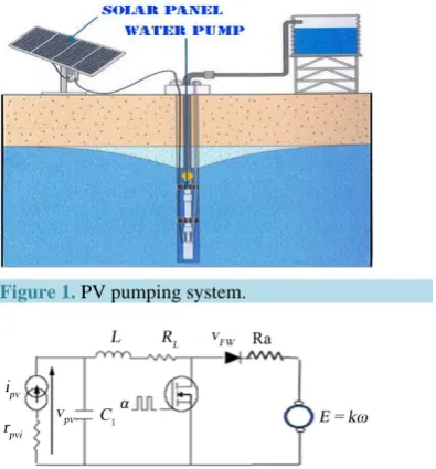
Based on these works, we propose in this paper a H∞ observer-based on tracking controller based on TS re-presentation of the PV pumping system, where the weighting functions depend on non-measurable premise va-riables [8]-[10]. Sufficient conditions, based on Lyapunov approach and the convex optimization techniques, are formulated as an efficient one step LMI [11] to avoid the complexity of separate design steps and can be solved using MATLAB software. The block diagram of a DC pumping system is shown in Figure 1 [12].

The structure of this paper is organized as follows. In Section II we describe the process of getting a T-S fuzzy model of PV system, with the DC motor pumping [13]. Section III presents the proposed control design. The stability conditions of the closed loop system are proposed in this section in terms of LMIs. In Section IV, we present the proposed strategy of the observer and the controller. In Section V, the simulation results are pre-sented and discussed. Finally, conclusions are made in Section VI.

2. Model of Pumping System

The water pumping system is considered in this work as a standalone system, without batteries. This is a com-plex and nonlinear system. The complete model is difficult to use in control applications. We need an easy mod-el to use for the synthesis of observers and controllers. It also allows estimating or adjusting the values of dy-namic parameters in real time. The system consists of a single PV module, an MPPT System, and a DC water pump. In the literature, different models of PV and of the pump were used. Figure 2 shows the equivalent circuit of the boost of the PV system with water pump.

The system [3] average model is given in (1):

(

)

(

)

2 1 d d d d d . d

pv a L fw a m L fw

L

L

pv pv L

L

v R R v R R i v kw

i k

i w u

t L L L L L

v i i

t C C

k k

w k k

u i w

t j j j j

 +  − + +  = − − − +  _ _      _{= −}      = − − −       (1)

where V_pv and i_pv refer to the PV panel voltage and current respectively. L, RL and iL are the self-in- ductance, resistance and current.Rm is a resistance characterizing IGBT lost.

C, VFW and ω are the input capacitance, the diode forward voltage and speed. u is the control input. Considering the PV current as an exogenous input, we get the state representation (2).

(

)

2 1

1

d 1

0 0 0 .

d

0

fw

a b

a m L fw

L L

pv

pv pv

L

v

R R k

R R i v k

L L L L

i i _L

i

v v u

t C C

k

k k

k i

j

j j j

ω ω ω ₋ +  ₋  _{ }   − + + −  _ _            _{ } _{  }    _{= −}  _{ +  +}        _{  }           _{ }   ₋  _{ }   − −           (2)

In order to guarantee zero steady state regulation error, we develop an integral T-S fuzzy control. Let Vref be

[image:3.595.229.427.86.299.2] [image:3.595.177.456.509.724.2]

Figure 1.PV pumping system.

Figure 2.Model of PV system with a motor-pump load.

(

ref

)

d

e pv

x =

∫

V −V t (3)

The new augmented state vector then becomes:

L pv e i V x x ω       =       (4)

So this second integrator included previous to the input would make it smoother, benefiting the implementa-tion, and therobustness [14].

The augmented system can be written as (5):

( )

w

x=Ax+B x u+B d (5)

where

(

)

1

0

1

0 0 0

0 0 0

0 1 0 0

a L

R R k

L L L

A C k j  +  − −       −   =          ₋    ;

( )

(

)

0 0

a m L FW

L

R R i V k

L B x k i j ω  − + +        =    ₋        1 1 pv ref i d V       =         ; 1

0 0 0

1

0 0 0

0 0 0

0 0 0 1

3. Control Strategy

In this work two control strategies are studied.

3.1. Perturb and Observe Algorithm

The P&P algorithm acts periodically by giving a perturbation to operating voltage V and observing the power variation P=V ii n order to deduct the direction of evolution to give to the voltage reference Vref. Taking into

account power-voltage characteristic curve p−v obtained under given conditions, the goal is to track the op-erating point at the MPP as shown in Figure 3. This algorithm measures at each z instant variable

( )

z and

( )

v z and calculates p z

( )

, then compares with the power calculated at

(

z−1

)

instant p z

(

−1

)

.

For all the operating points where the power and current variations are positive, the algorithm that continued to perturb the system in the same direction of perturbation is reversed. The increasing of reference voltage Vref,

otherwise, if these variations are negative, the direction of perturbation is reversed. The increasing or decreasing of reference Vref is done by tracking step ∆V . The flow chart of the P&O algorithm is presented in Figure 4.

Theoretically, the algorithm is simple to implement in its basic form. However, it was noticed some oscillations around the MPP in steady state operating and this causes power loss [15]. Its functioning depends on the track-ing step size applied to voltage reference Vref. For the same sample time of the system, the oscillations and

[image:4.595.191.448.324.449.2]

consequently the power loss could be minimized if the tracking step would continuously get smaller [16]. Nev-ertheless, the response of the algorithm becomes slower.

Figure 3.Power-Voltage characteristic of PV panel.

[image:4.595.173.456.480.708.2]

3.2. Takagi-Sugino Fuzzy Model

In this section, we present T-S fuzzy control approach that ensures robust regulation under disturbance. Consider a general nonlinear system as follows:

( )

1

2

w

x Ax B x u B d

z C x

y C x

= + +   =   =   (6)

z is the controlled output variable and y is the output vector.

By observing the functions of A x

( )

, B x

( )

, the fuzzy premise variables are chosen as z1 =iL and z2 =ω.

Then, the system (2)-(5) can be represented by the following T-S fuzzy rules: IFz t1

( )

is F1i and z2 is F2i, then [17].

( )

( )

( )

1

2

1, 2, , . w

x Ax B x u B d

z t C x i r

y t C x

= + +

= =

=



 (7)

where Fji

(

j=1, 2

)

are the fuzzy sets, r is the number of fuzzy rules, and Ai, Bi, C1, and C2 are

appro-priate subsystem matrices.

The global T-S model is then inferred as follows:

( )

(

)

( )

( )

4 1 1 2

i i w

i

x t Ax B u B d

z t C x y t C x

µ =  _{= + +}   ₌   ₌  

∑

 (8)

where h t

( )

= _z t₁

( )

z₂

( )

t _T,

(

( )

)

(

( )

)

( )

(

)

1 0 i i r i i

w h t h t

w h t µ

=

= ≥

∑

, with

(

( )

)

(

( )

)

2

1

i ji i

j

w h t F z t

=

=

∏

so that

( )

(

)

1 1

r i

i= µ h t =

∑

for all t. To obtain an exact fuzzy representation of dynamic (2), the membership functions of z1 and z2 should be chosen so that 1

(

( )

)

r i

i t Ai

A=

∑

₌ µ h and B x

( )

=

∑

ir=₁µi

(

h t

( )

)

Bi. For simplification,

let us write the membership function in the general form [18].

( )

1

1 .

j

aj j bj aj

j j j j

d

S z t S S

D d D d

 

−

= +_ _ = −

− _ − _

where Dj ≡maxx∈Ω_x zj

( )

t and dj ≡minx∈Ωx zj

( )

t , for j=1, 2 and the discussion set:

(

)

[

]

{

, min, max , for 1, 2

}

x x iL ω xi i

Ω ≡ = ∈   = . (Note that lmin and lmax are the lower and upper bounds of

variable xi respectively).

Hence, functions µ_i

(

h t

( )

)

are the weighting functions depending on variable h t

( )

which can be measur-able (as the input or the output of the system) or unmeasurmeasur-able varimeasur-ables [19] [20] (as the state of the system) and verify the following properties:

( )

(

)

( )

(

)

{

}

4

1 1 _{1, , 4}

0 1 i i i i h t h t µ µ =  ₌  _{∀ ∈}  ≤ ≤ 

∑

_

(7) becomes:

( )

4

(

( )

)

(

)

( )

( )

( )

2 1

ˆ

i i i w

i

x t µ x t A x B u B d w t y t C x t

=

=

∑

+ + + =

 　　　 (9)

where

( )

(

(

( )

)

(

( )

)

)

(

)

4

1

ˆ

i i i

i w

i

w t µ x t µ x t A x Bu B d

=

=

∑

− + + .

4. Fuzzy Observer Based Tracking Controller

The aim of this section is the design of the observer-based tracking control of the photovoltaic Pumping System. As the motor speed model states are not fully measurable, the designed state feedback control is based on the es-timated states. We define the fuzzy controller as follows:

( )

4

(

( )

)

(

( )

)

1

ˆ _iˆ

i

i x t

u t µ K x t

=

=

∑

(10)

where x tˆ

( )

∈ℜ4 is the estimated state and Ki 1 4 ×

∈ℜ

(

i=1,, 4

)

are the controller gains to be determined. Based on T-S fuzzy model of solar pump (1), the structure of the observer is defined as:

( )

4

(

( )

)

(

( )

(

)

)

( )

( )

.

2 1

ˆ _i ˆ _iˆ _{i i} ˆ ˆ ˆ

i

x t µ x t A x t B u L y y y t C x t

=

=

∑

+ + − 　　 = (11)

where y tˆ

( )

∈ℜ3 is the estimated output, Li 4 3 ×

∈ℜ

(

i=1,, 4

)

are the observer gains to be determined. Let’s define error of state estimation as e0

( ) ( ) ( )

t =x t −xˆ t ; then, we can find the estimation error dynamics

as follows:

( )

4

(

( )

)

(

(

) ( )

)

( )

0 2 0

1 ˆ

i i i w

i

e t µ x t A L C e t B d w t

=

=

∑

− + +

 (12)

Augmented system

( )

( )

0 t t x x e   =    

 ; can be written as

( )

(

)

(

( )

)

(

( )

( )

)

( )

( )

4 4 1 1 2

ˆ ˆ ˆ

i j ij i

i i

x x t x t A x t H w t

y t C x t

µ µ = = = + =

∑ ∑

    

  (13)

with

2

0

i i j i j

ij

i i

A B K B K

A

A L C

−   =  ₋   ; 4 4 w i w B I H B I   =    ; d w w   =  

 ; C2 =

[

C2 4

]

.

The estimation error asymptotically converges around zero and satisfies the following H∞ performance un-der zero initial conditions:

( )

( )

( )

0 ₂

2

, for 0. e

w w

t

t

t ≤γ ≠ (14)

where γ is the desired disturbance attenuation parameter.

Theorem 1: if there exists symmetric matricesX1>0, P2 >0, matrices Y Ji i and a prescribed

2

0

γ > , such that the following LMI holds [21]:

2 2 2

2

2

0 0 0

* 2 0 0 0 0

* * 2 0 0 0

0

* * * 2 0 0

* * * *

* * * * * 0

* * * * * *

ij i j w

ij w

B Y B I

I I

I I

I I

P B P

I I µ µ µ µ µ µ γ γ Λ    ₋     −   _{−  ≤}  

 _Γ 

where

T T T

1 1

ij A Xi X Ai B Yi j Y Bj i

Λ = + − − (16)

Controller gains Ki and observer gains Li are given by:

1 1

i i

K =Y X− (17)

1

2 1

i

L =P J− (18)

Proof

Consider the following Lyapunov function candidate:

( )

(

)

T

( ) ( )

T

, 0.

V x x =x t Px t P=P > (19)

The time derivate of V x t

(

( )

)

(12) is given by

( )

(

)

4 4

(

( )

)

(

( )

)

T

( )

(

T

)

( )

T

( )

( )

T

( )

T

( )

1 1

ˆ ˆ .

i j ij ij i i

i i

V x t µ x t µ x t x t PA A P x t x t PH w t w t H Px t

= =

 

=

∑∑

_  +   +   +    _

The closed loop system with controller-based observer is stable and has H∞ norm limited by γ if and only if:

( )

(

)

T

( ) ( )

2 T

( ) ( )

0 0 0

V x t  +e t e t −γ w t w t < (20)

Therefore, we have

( )

(

)

(

( )

)

T

4 4

1 1 i ˆ j ˆ ij 0

i j x x x x w w t t µ µ = =

  _Ξ  _≤

   

   

∑ ∑

_ _ (21)

where

T T

2 4 *

ij ij i

ij

A P PA I I PH

I γ

 + + 

Ξ =  ₋ 

 

    

, I=

[

0 I4

]

.

Inequality (19) is satisfied if condition 20 holds:

0

ij

Ξ ≤ (22)

Let us consider thefollowing particular form of 1

2 0 0 P P P   =    , T

1 1 0

P =P > , P2=P2T>0 Then after simple

manipulation, inequality (17) can be reformulated as:

1 1 1 1

2 2 2

2 4

2 4

*

* * 0

* * *

ij i j w

ij w

ij

P B K P B P

P B P

I I γ γ Γ  

 _Γ 

  Ξ =  −   ₋    (23) with

(

) (

)

T

1ij P A1 i B Ki j Ai B Ki j P1

Γ = − + − and Γ =_2ij P A₂

(

_i−L C_{i 2}

) (

+ A_i−L C_{i 2}

)

TP₂+I₄.

It should be noted that condition (18) is nonlinear with respect variables P1 and K2 Then, the objective is

to formulate (18) in LMI constraints.

Hence, after partitioning the matrix inequality shown in (18), Ξij becomes:

11 12 22 * ij Ξ Ξ  

Ξ =  _Ξ 

  (24)

12

Ξ is the upper right block of (22) and Ξ22 is the lower right block of (22).

1

1 0

0 P Q

X

−

 

=  

  and

1

1 0

0 P X

I

−

 

=  

 

Post and pre-multiplying inequality (21) by Q, it follows that (23) can be rewritten as:

1 1 1

1 11 1 1 12

22 0 *

P P P X

X X

− − −

 Ξ Ξ _≤

 _Ξ 

  (25)

Lemma 2: Considering Ξ ≤22 0 a matrix X and a scalar µ, the following holds [21] [22]:

(

₁

)

T

(

₁

)

_{2 1}

22 22 22 0 22 2 22

X+ Ξµ − Ξ X+ Ξµ − ≤ ⇔ ΞX X ≤ − µX−µ Ξ− (26)

By substituting (22) into (21) and using the Schur complement, then inequality (21) holds if (23), displayed below, is satisfied:

1 1 1

1 11 1 1 12

22 0

* 2 0

* *

P P P X

X I

µ µ

− − −

 Ξ Ξ 

 ₋ _≤

 

 _Ξ 

 

(27)

By changing matrices Ξ11,Ξ12 and Ξ22 by their expressions from (19) and considering

1

1 1

X =P− ,

1

j j

Y =K X we obtain an LMI in (14).

5. Simulation Results

[image:8.595.190.441.519.707.2]

To illustrate the proposed method, the Observer based robust controller law is tested by considering the T-S Model of the photovoltaic pumping. The controller is tested by simulation. This section shows the efficiency of the designed control of system through computer simulations.

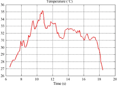
Figure 5 and Figure 6 present the climatic conditions on one day (temperature and solar irradiance). To validate our approach, we compare these results with those given by the classical P&O method.

In Figure 7, the simulation result shows that the power obtained in our case is better than using the P&O me-thod.

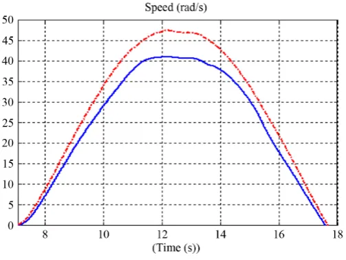
Figure 8 shows the comparison of motor speed using the two methods. We can see the difference and the im-portance of our approach.

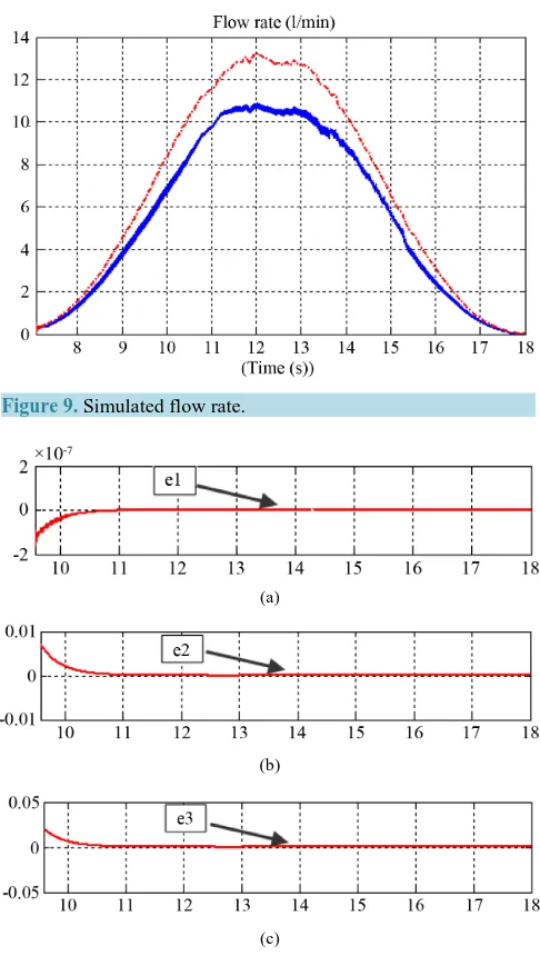
Finally, the water flow obtained by the two methods is presented in Figure 9.

The errors of state estimation are given in Figure 10, where all errors asymptotically converge to zero. The Simulation results showing the confusion of the P&O algorithm with reference voltage perturbation by a step increase in solar irradiance (Figure 11).

[image:9.595.185.445.90.269.2] [image:9.595.189.441.519.708.2]

Figure 6.The solar irradiance for a day.

Figure 7.Maximum power obtained by two methods.

[image:10.595.191.434.81.511.2]

Figure 9.Simulated flow rate.

(a)

(b)

[image:10.595.198.434.549.704.2]

(c)

Figure 10.Estimation error of (a) inductance current; (b) PV array Voltage; and (c) Motor speed.

6. Conclusion

In this paper, a robust H∞ observer-based tracking control of the photovoltaic Pumping System has been pro-posed. The designed controller ensures the optimum of power and guarantees a better flow of water. The stabili-ty conditions are given in terms of LMIs, which can be solved in one single step-procedure to determine the ob-server and the controller gains. From simulation results, the performances of the designed robust obob-server-based controller are satisfactory and the capability of this controller is shown under critical situations. To put that in perspective, we will test this control law on a test branch that we are developing in our laboratory.

References

[1] Arrouf, M. (2007) Optimisation de l’Ensemble Onduleur, Moteur et Pompe, Branches sur un Genérateur Photo- voltaïque. Thèse de Doctorat, Université Mentouri de Contrainte, Constantine.

[2] Khalil, H.K. (2000) Universal Integral Controllers for Minimum-Phase Nonlinear System.IEEE Transactions on Au-tomatic Control, 45, 490-494.

[3] Elgendy, M.A., Zahawi, B. and Atkinson, D.J. (2012) Assessment of Perturb and Observe MPPT Algorithm Imple- mentation Techniques for PV Pumping Applications. IEEE Transactions on Sustainable Energy, 3, 21-23.

[4] Elgendy, M.A., Zahawi, B. and Atkinson, D.J. (2010) Comparison of Directly Connected and Constant Voltage Con-trolled Photovoltaic Pumping Systems. IEEE Transactions on Sustainable Energy, 1, 184-192.

[5] Hadji Arab, A., Benghanem, M. and Chenlo, F. (2006) Motor-Pump System Modelization. Renewable Energy, 31, 905- 913.

[6] Elgendy, M.A., Zahawi, B. and Atkinson, D.J. (2008) Analysis of the Performance of DC Photovoltaic Jumpings Sys-tems with Maximum Power Point Tracking. IET International Conference on Power Electronics, Machines and Drives, York, 2008, 426-430.

[7] Akbaba, M. (2006) Optimum Matching Parameters of an MPPT Unit Based for a PVG-Powered Water Pumping Sys-tem for Maximum Power Transfer.International Journal of Energy Research, 30, 395-409.

http://dx.doi.org/10.1002/er.1157

[8] Ghorbel, H., Souissi, M., El Hajjaji, A. and Chaabane, M. (2011) Design of Multi-Observers for Takagi-Sugeno Sys-tems with Unmeasurable Premise Variables: Descriptor Approach. International Conference on Sciences and Tech-niques of Automatic Control and Computer Engineering (STA), Sousse, 18-20 December 2011, 250-256.

[9] Ichalal, D., Marx, B., Ragot, J. and Maquin, D. (2009) State Estimation of Nonlinear Systems Using Multiple Model Approach. American Control Conference (ACC), St. Louis, 10-12 June 2009, 4636-4641.

[10] Nagy, A., Marx, B., Mourot, G., Schutz, G. and Ragot, J. (2010) State Estimation of Two-Time Scale Multiple Models with Unmeasurable Premise Variables. Application to Biological Reactors. 49th IEEE Conférences on Décisions and Control, 15-17 December 2010, 5689-5694.

[11] Oudghiri, M., Chadli, M. and El Hajjaji, A. (2007) One-Step Procedure for Robust Output H1 Fuzzy Control. 15th Mediterranean Conference on Control and Automation,Athens, 27-29 June 2007, 1-6.

[12] Ouachani, I., Rabhi, A., El Hajjaji, A., Tidhaf, B. and Zouggar, S. (2013) A Robust Control Method for a DC Mo-tor-Based Photovoltaic Pumping. Proceedings of the 3rd International Conference on System and Control, Algiers, 29-31 October 2013, 720-726.

[13] Ouachani, I., Rabhi, A., Tidhaf, B., Zouggar, S. and Elhajjaji, A. (2013) Optimization and Control for a Photovoltaic Pumping System. 2nd International Conference on Renewable Energy Research and Applications, Madrid, 20-23 Oc-tober 2013, 734-739.

[14] Lian, K.-Y., Ouyang, Y.-L. and Wu, W.-L. (2008) Realization of Maximum Power Tracking Approach for Photovol-taic Array Systems Based on T-S Fuzzy Method. IEEE International Conference on Fuzzy Systems, Hong Kong, 1-6 June 2008, 1874-1879.

[15] Takagi, T. and Sugeno, M. (1985) Fuzzy Identification of Systems and Its Applications to Modeling and Control. IEEE Transactions on Systems, Man and Cybernetics, SMC-15, 116-132. http://dx.doi.org/10.1109/TSMC.1985.6313399 [16] Chiu, C.-S. (2010) T-S Fuzzy Maximum Power Point Tracking Control of Solar Power Generation Systems. IEEE

Transactions on Energy Conversion, 25, 1123-1132.

[17] Ichalal, D., Marx, B., Ragot, J. and Maquin, D. (2007) Conception de multi-observateurs variables de décision non mesurables. 2 Journes Doctorales/Journes Nationales MACS, Reims.

[18] Boyd, S., El Ghaoui, L., Feron, E. and Balakrishnan, V. (1994) Linear Matrix Inequalities in System and Control Theory. SIAM, Philadelphia. http://dx.doi.org/10.1137/1.9781611970777

National Polytechnique de Lorraine, Frensh.

[20] Guerra, T., Kruszewski, A., Vermeiren, L. and Tirmant, H. (2006) Conditions of Output Stabilization for Nonlinear Models in the Takagi-Sugeno’s Form. Fuzzy Sets and Systems, 157, 1248-1259.

http://dx.doi.org/10.1016/j.fss.2005.12.006

[21] Tafticht, T., Agbossou, K., Doumbia, M.L. and Cheriti, A. (2008) An Improved Maximum Power Point Tracking Me-thod for Photovoltaic Systems. Renew Energy, 33, 1508-1516. http://dx.doi.org/10.1016/j.renene.2007.08.015