Evaluation of Neural Pattern Classifiers for a Remote Sensing Application

Munich Personal RePEc Archive

Evaluation of Neural Pattern Classifiers

for a Remote Sensing Application

Fischer, Manfred M. and Gopal, Sucharita and Staufer,

Petra and Steinnocher, Klaus

Vienna University of Economics and Business, Boston University,

Vienna University of Economics and Business, Vienna University of

Economics and Business

1995

Online at

https://mpra.ub.uni-muenchen.de/77811/

Abteilung fi.ir Theoretlsche und Angewandte Wlrtschafts- und Sozialgeographie

lnstltut fi.ir Wirtschafts- und Sozlalgeographie

Wirtschaftsuniversitat Wien

Vorstand: o.Univ.Prof. Dr. Manfred M. Fischer

A - 1090 Wien, Augasse 2-6, Tel. (0222) 313 36 - 4836

Redaktion: Mag. Petra Staufer

WSG 46/95

Evaluation of Neural Pattern Classifiers

for a Remote Sensing Application

Manfred M. Fischer, Sucharita Gopal, Petra Staufer and Klaus Steinnocher

Gedruckt mit Unterstutzung des Bundesministerium tor Wissenschaft und Forschung

in Wien

WSG Discussion Papers are interim reports presenting work in progress and papers which have been submitted

Abstract

This paper evaluates the classification accuracy of three neural network classifiers on a satellite

image-based pattern classification problem. The neural network classifiers used include two types

of the Multi-Layer-Perceptron (MLP) and the Radial Basis Function Network. A normal

(conventional) classifier is used as a benchmark to evaluate the performance of neural network

classifiers. The satellite image consists of 2,460 pixels selected from a section (270 x 360) of a

Landsat-5 TM scene from the city of Vienna and its northern surroundings. In addition to

evaluation of classification accuracy, the neural classifiers are analysed for generalization capability

and stability of results. Best overall results (in terms of accuracy and convergence time) are

provided by the MLP-1 classifier with weight elimination. It has a small number of parameters and

requires no problem-specific system of initial weight values. Its in-sample classification error is

7.87% and its out-of-sample classification error is 10.24% for the problem at hand. Four classes of

simulations serve to illustrate the properties of the classifier in general and the stability of the result

with respect to control parameters, and on the training time, the gradient descent control term,

initial parameter conditions, and different training and testing sets.

Keywords: Neural Classifiers, Classification of Multispectral Image Data, Pixel-by-Pixel

1. Introduction

Evaluation of Neural Pattern Classifiers

for a Remote Sensing Application

Satellite remote sensing, developed from satellite technology and image processing, has been a

popular focus of pattern recognition research since at least the 1970s. Most satellite sensors used for

land applications are of the imaging type and record data in a variety of spectral channels and at a

variety of ground resolutions. The current trend is for sensors to operate at higher spatial resolutions

and for providing more spectral channels to optimize the information content and the usability of

the acquired data for monitoring, mapping and inventory applications. At the end of this decade, the

image data obtained from sensors on the currently operational satellites will be augmented by new

instruments with many more spectral bands on board of polar orbiting satellites forming part of the

Earth Observing System (Wilkinson et al. 1994).

As the complexity of the satellite data grows, so too does the need for new tools to analyse them in

general. Since the mid 1980s, neural network (NN) techniques have raised the possibility of

realizing fast, adaptive systems for multispectral satellite data classification. In spite of the

increasing number of NN-applications in remote sensing (see, for example Key et al. 1989,

Benediktsson et al. 1990, Hepner et al. 1990, Lee et al. 1990, Bischof et al. 1992, Beerman and

Khazenie 1992, Civco 1993, Dreyer 1993, Salu and Tilton 1993, Wilkinson et al. 1994) very little

has been done on evaluating different classifiers. Given that pattern classification is a mature area

and that several NN approaches have emerged in the last few years, the time seems to be ripe for an

evaluation of different neural classifiers by empirically observing their performance on a larger data

set. Such a study should not only involve at least a moderately large data set, but should also be

unbiased. All the classifiers should be given the same feature sets in training and testing.

This paper addresses the above mentioned issue in evaluating the classification accuracy of three

neural network classifiers. The classifiers include two types of the Multi-Layer Perceptron (MLP)

and a Radial Basis Function Network (RBF). The widely used normal classifier based on

parametric density estimation by maximum likelihood, NML, serves as benchmark. The classifiers

were trained and tested for classification (8 a priori given classes) of multispectral images on a

pixel-by-pixel basis. The data for this study was selected from a section (270 x 360 pixels) of a

In section two of this paper, we will describe the structures of the various pattern classifiers. Then

we will describe the experimental set-up in section 3, i.e. the essential organization of inputs and

outputs, the network set-ups of the neural classifiers, a technique for addressing the problem of

overfitting, criteria for evaluating the estimation (in-sample) and generalization (out-of-sample)

ability of the different neural classifiers and the simulation set up (section 3). Four classes of

simulations serve to analyse the stability of the classification results with respect to training time

(50,000 epochs), the gradient descent control term (constant and variable learning schemes), the

initial parameter conditions, and different training and testing sets. The results of the experiments

are presented in section 4. Finally, in section 5 we give some concluding remarks.

2. The Pattern Classifiers

Each of our experimental classifiers consists of a set of components as shown in figure 1. The ovals

represent input and output data, the rectangles processing components, and the arrows the flow of

data. The components do not necessarily correspond to separate devices. They only represent a

separation of the processing into conceptual units so that the overall structure may be discerned. The inputs may - as in the current context - come from Landsat-5 Thematic Mapper (TM) bands.

Figure 1: Components of the Pixel-by-Pixel Classification System

Input Pixels

Discriminant ~ Maximum

Functions Finder

Hypothesized Class

Each classifier provides a set of discriminant functions De (l:::;;c:::;;C, C number of a priori given

classes). There is one discriminant function De for each class c. Each one provides a single

floating-point-number which tends to have a large number if the input pixel (i.e. feature vector x of

the pixel, x E 9tn) is of the class corresponding to that particular discriminant function. The C-tuple

of values produced by the set of discriminant functions is sent to the 'Maximum Finder'. The

'Maximum Finder' identifies which one of the discriminant values Dc(x) is highest, and assigns its

class as the hypothesized class of the pixel, i.e. uses the following decision rule

Assign x to class c if Dc(x) >Dk (x) for k=l, ... , C and k '# c (1)

Three experimental neural classifiers are considered here: multi-layer perceptron (MLP) classifiers

classifier NML serves as statistical benchmark. The following terminology will be used in the

descriptions of the discriminant functions below: .

n dimensionality of feature space (n representing the number of spectral bands used, n=6 in our

application context),

9tn the set of all n-tuples of real numbers (feature space),

x feature vector of a pixel (x = (x1, ... , xn) e 9tn),

C number of a priori given classes (l~c~C).

2.1 The Normal Classifier

This classifier (termed NML) which is most commonly used for classifying remote sensing data

serves as benchmark for evaluating the neural classifiers in this paper. NML is based on parametric

density estimation by maximum likelihood (ML). It presupposes a multivariate normal distribution

for each class c of pixels. In this context, it may be worthwhile to mention first factors pertaining to

any parametric classifier.

Let L(clk) denote the loss (classification error) incurred assigning a pixel to class c rather than to

class k. Let us define a particular loss function in terms of the Kronecker symbol Dck

c=k

otherwise (2)

This loss functilln implies that correct classifications yield no losses, while incorrect classifications

produce equal loss values of 1. In this case the optimal or Bayesian classifier is that one which

assigns each input x ('feature vector' of a pixel), to that class c for which the a posteriori probability

p( clx) is highest, i.e.

p(c Ix) ;::: p(k Ix)

According to Bayes rule

p(c Ix)

=

I

k=l, ... ,C (5)

(4)

where p(c) denotes the a priori probability of class c and p(x) the mixture density

f

probabilities are the same, p( c) can be ignored. For the normal classifier NML each class c is

assumed to have a conditional density function

c= l, .. ., C (5)

with

µc

right-hand side of (5) is constant and may be discarded for classification. By replacing the mean

vectors

µc

taking logarithms the set of NML-discriminant functions is given by

(6)

where

p(

2.2 The Multi-Layer Perceptron Classifiers

Multi-layer perceptrons are feed-forward networks with one or more layers of nodes between the

input and output nodes. These additional layers contain hidden (intermediate) nodes or units. We

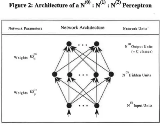
have used MLPs with three layers (counting the inputs as a layer), as outlined in figure 2.

Figure 2: Architecture of a N(O) : N(l) : N(2) Perceptron

Network: Parameters

(2)

Weig hts O)cj

<Ji' )

W e ights j i

Network Architecture Network Units ·

(2)

N Outpu t Unit s

(= C classes)

(I)

N Hidden Units

(0)

N Input Un its

Let N(k) denote the number of units in the k-th 11;1yer (k = 0, 1, 2). The number of inputs, N<0>[=n]

six for the input layer (one for each spectral channel TMl, TM2, TM3, TM4, TM5 and TM7) and

eight for the output layer (representing the eight a priori categories of the pixels). The parameter with respect to the network architecture outlined in figure 2 is the number N(l) of non-linear hidden

units that are fully connected to the input units and with the output units. Output and hidden units

have adjustable biases (left out of consideration in figure 2). The weight

mjJ)

of the (1-1)-th layer to the j-th node of the I-th layer (1=1, 2; 1 ~ i ~ ~I-1), 1 ~j~ ~ 0 ). The weights

can be positive, negative or zero.

Let us define

b~

)

hidden unit activation function, then the set of discriminant functions are of the form:

N(l) N(O)

exp{b(2)

+

+

x-)}

C j=I CJ J i=I JI l

Dc(x)

=

(7)

L

+

L

+

L

1=1 I j=l lj "f' J . k=I jk k

It is worthwhile to note that classifiers of type (7) use a softmax output unit activation function (see

Bridle 1989). This activation function is a composition of two operators: an exponential mapping, followed by a normalisation to ensure that the output activations are non-negative and sum to one.

The specification of the activation function 'I' is a critical issue in successful application

development of a MLP classifier. We have experimented with two types of sigmoid functions, the

most widely used non-linear activation functions: asymmetric and symmetric sigmoid functions.

We use logistic activations for defining MLP-1 and hyperbolical tangent (tanh) activations for MLP-2.

The activation Sh of a logistic (sigmoid) hidden unit is given by

(8)

which performs a smooth mapping (-oo, +oo) ~ (0,1). The slope 'a' can be absorbed into weights

and biases without loss of generality and is set to one.

The activation Th of a tanh hidden unit is given by

performing a smooth mapping (-oo, -too) -7 (-1, +1). We here also set a=l.

For the training of the weights of MLP networks, a reasonable procedure is the use of an

optimization algorithm to minimise the mean-square-error (least mean square error function) over

the training set between the discriminant values actually produced and the target discriminant

values that consist of the appropriate strings of ls and Os as defined by the actual classes of the

training pixels. For example, if a training vector is associated to class 1, then its target vector of

discriminant values is set to (1,0, ... , 0).

Networks of the MLP type are usually trained using the error backpropagation algorithm (see

Rumelhart et al. 1986). Error backpropagation is an iterative gradient descent algorithm designed to

minimise the least square error between the actual and target discrimination values. This is

achieved by repe_atedly changing the weights of the first and second parameter layer according to the gradient of the error function. The updating rule is given by

(k) (k)

a

rors (t+ 1) = rors (t)

+

~ rors

k=l,2 (10)

Where E denotes the least mean square error function to be minimised over the set of training

examples, and 11 the learning rate, i.e. the fraction by which the global error is minimised during

each pass. The bias value bh is also learned in the same way. In the limit, as 11 tends to zero and the number of iterations tends to infinity, this learning procedure is guaranteed to find the set of

weights which gives the least mean square error (see White 1989).

2.3 The Radial Basis Function Classifier

In the MLP classifiers, the net input to the hidden units is a linear combination of the inputs. In a

Radial Basis Function (RBF) network the hidden units compute radial basis functions of the inputs.

The net input to the hidden layer is the distance from the input to the weight vector. The weight

vectors are also called centres. The distance is usually computed in the euclidean metric. There is

generally a bandwidth

a

units can be any of a variety of functions on the non-negative real numbers with a maximum at

zero, approaching zero at infinity, such as the Gaussian transfer function.

We have experimented with a RBF classifier which uses softmax output units and Gaussian

(k) (k) (k)

)T

C = (cl , .. ., Cn E

':Jt

denote the centre vector of the k-th hidden unit and

(k) (k) (k)

)T

cr = _{(cr 1 , ... ,crn} e 9t

(1)

k=l, ... ,N

(1)

k=l, ... ,N

its width vector, while

b~I)

ro}~)

respectively.

Then the discriminant functions are given by:

N(I)

exp{b(2) + Lro(2) ..i. (x)}

c k=l ck 't'k

Dc(x) = - - - -_{Nc2i N(I)}

L

b~

)

L

co~)

l=I k=l

where each hidden unit j computes the following radial basis function:

(

N(O) (

(k) J2J

(k) J2J

<l>k(x) =exp

-L

•=I <J.·(k) i=t cr~k)

I I

c=l, ... , C

(I) k=l, ... ,N

(11)

(12)

The centres c(k), widths cr(k), output bias nodes b?) and output node weights

co}~)

considered as trainable weights of the RBF network. They are trained initially using the cluster

means (obtained by means of the K-means algorithm) as the centre vectors c(k). The width vectors

cr(k) are set to a single tunable positive value. Note that no target discriminant values are used to

determine c(k) and cr(k), while training of the output weights and bias proceeds by optimization

identical to that described for the MLP classifiers.

The crucial difference between the RBF and the two MLP classifiers lies in the treatment of the

inputs. For the RBF classifier, as can be seen from (12), the inputs factor completely. Unless all

inputs xi (1 :5 i :5 n) are reasonably close to their centres c}k)' the activation of hidden unit k is close

to zero. A RBF unit is shut off by a single large distance between its centre and the input in any one

of the dimensions. In contrast, in the case of the MLP classifiers, a large contribution by one

weighted output in the sum of (7) or (8) can often be compensated for by the contribution of other

3. Experimental Set up

3.1 The Data and Data Representation

The data used for training and testing the classification accuracy of the classifiers was selected from

a section (270 x 360 pixels) of a Landsat-5 Thematic Mapper (TM) scene. The area covered by this

imagery is 8. lxl0.8 km2 and includes the city of Vienna and its northern surroundings. The spectral

resolution of each of the six TM bands (TMl, TM2, TM3, TM4, TM5, TM7) which were used in

this study was eight bits or 256 possible digital numbers. Each pixel represents a ground area of

30x30 m2. The purpose of the multispectral image classification task was to distinguish between

eight land cover categories as outlined in table 1.

One of the authors, an expert photo interpreter with extensive field experience of the area covered

by the image, used ancilliary information from maps and orthophotos (from the same time period)

in order to select suitable training sites for each class. One training site was selected for each of the

eight categories of land cover [single training site case]. This approach resulted in a database

consisting of 2,460 pixels (about 2.5 percent of all the pixels in the scene) that are described by

six-dimensional feature vectors and their class membership (target values). The set was divided into a

training set (two thirds of the training site pixels) and a testing set by stratified random sampling,

stratified in terms of the eight categories. Thus each training/test run consists of 1,640 training/820

testing vectors. This moderately large size for each training run makes the classification problem

non-trivial at the one hand, but still allows for extensive tests on in-sample and out-of-sample

performance of the classifiers.

Table 1: Categories Used for Classification and Number of Trainingffesting Pixels

Category Description of the Category Pixels

Number Training Testing

CI Mixed grass and arable farmland 167 83

C2 Vineyards and areas with low vegetation cover 285 142

C3 Asphalt and concrete surfaces 128 64

C4 Woodland and public gardens with trees 402 200

cs

C6 Densely built up residential areas (urban) 296 148

C7 Water courses 153 77

cs

Data preprocessing (i.e. filtering or transforming the raw input data) plays an integral part in any

classification system. Good preprocessing techniques reduce the effect of poor quality (noisy) data

and this usually results in improved classification performance. In this study, the classifiers

implemented in the experiments use gray coded data. The gray scale values in each spectral band were linearly compressed in the (0.1, 0.9) range to generate the input signals.

3.2 Network Set Up of the Neural Classifiers and the Overfitting Problem

The architecture of a neural classifier is defined by the arrangement of its units, i.e. the set of all

weighted connections between units (see figure 2). This arrangement (i.e. the topology) of the

network of a classifier is very important in determining its generalization ability. Generalization

refers to the ability of a classifier to recognize patterns outside the training set. An important issue

for good generalization is the choice of the optimal network size. This means finding the optimal

number of hidden units, since inputs and outputs are defined by the problem at hand. There are

some rules of thumb which often fail drastically since they ignore both the complexity of the task at

hand and the redundancy in the training data (Weigend 1993). The optimal size of the hidden layer

is usually not known in advance.

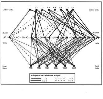
Figure 3: The Pruned MLP-1with14 'Degrees of Freedom' and 196 Parameters

Output Units

Hidden

Units

Input

Units

CI C2 C3

TMI TM 2 TM4

Strengths or the Conoecdon Weights

I H U l l H l l l l l H > 5

- - - 0~5

C7 C 8

< -5

The number of hidden units when the minimum is arrived may be viewed as a kind of measure of

the degree of freedom of the network (Gershenfield and Weigend 1993). If the hidden layer is

chosen to be too small, it will not be flexible enough to discriminate the patterns well, even in the

training set. If it is chosen too large, the excess freedom will allow the classifier to fit not only the

signals, but also the noise. Both, too small and too large hidden layers thus lead to a poor

generalization capability in the presence of noise (Weigend et al. 1991).

This issue of overfitting or in other words the problem of estimating the network size has been

widely neglected in remote sensing applications, up to now. Recently, several techniques have been

proposed to get around this problem. To be relieved from the uncertainty of a specific choice of a

validation set of the cross-validation approach (see Fischer and Gopal 1994) we have chosen in this

study another approach, a network pruning or weight-elimination technique to overcome the

problem of overfitting. This technique starts with an oversized network and attempts to minimise

the complexity of the network (in terms of connection weights) and the standard sum squared error

function by removing 'redundant' or least sensitive weights (see Weigend et al. 1991).

We deliberately have chosen an oversized, fully connected MLP-1 network with 22 hidden units

and a variable learning rate. The 338 weights were updated after each 3 patterns, presented in

random order (stochastic approximation). In the first 17 ,000 epochs, the procedure eliminated the

weights between the eight output units and eight hidden units. Since these eight units did not

receive the signals in the backward pass anymore, their weights to the input subsequentially

decayed. In this sense, the weight-elimination procedure can be thought of as unit-elimination,

removing the least important hidden units. The weights and biases of the pruned MLP with 14

remaining hidd~n units are given in appendix A. The architecture of the pruned MLP-1 is outlined

in figure 3. The size of the network declined from 338 to 196 free parameters.

In contrast to MLP-classifiers, RBF networks are self-pruning to some degree. Unimportant

connections are effectively pruned away by the training process leaving a large width. Each large

width effectively deletes one connection from an input to one RBF and reduces the number of

active patterns by two.

3.3 Performance Measures

The ultimate performance measure for any classifier is its usefulness to provide accurate

classifications. This involves in-sample and out-of-sample classification accuracy. Four standard

• the classification error (also termed confusion) matrix (f_1k) with f_1k (l,k=l, ... , C) denoting the

number of pixels assigned by the classifier to category 1 and found to be actually in (ground

truth) category k,

• the map user's classification accuracy,'\\• for the ground truth category k=l, .. ., C

Uk

-

f.k -

-c--I:

i=l 1

• the map producer's classification accuracy 1t₁ for the classifier's category 1=1, .. ., C

1t1

f u f u

(14)

-f1.

-

-I:

j=l J

• the total classification accuracy 't [or the total classification error 't' defined as 't' = (100 -'t)]

c

L.

1"1 II

'C _{.- f ••}

c :Ef..

i"I II

.- c c

I:I:

l=l Jk

3.4 Experimental Simulation Set Up

(15)

Neural networks are known to produce wide variations in their performance properties. This is to

say that small changes in network design, and in control parameters such as the learning rate and the initial parameter conditions might generate large changes in network behaviour. This issue,

which is the major focus of our simulation experiments, has been highly neglected in remote

sensing applications up to now. In real-world applications, it is, however, a central objective to

identify intervals of the control parameters which give robust results, and to demonstrate that these

results persists across different training and test sets.

In-sample and out-of-sample performance are the two most important experimentation issues in this

study. In-sample performance of a classifier is important because it determines its convergence

ability and sets a target of feasible out-of-sample performance which might be achieved by

fine-tuning of the control parameters (Refenes et al. 1994). Out-of-sample performance measures the

ability of a classifier to recognize patterns outside the training set, i.e. in the testing set strictly set

• the gradient descent control term,

• initial parameter conditions, and

• training and testing sets.

Consequently, it is important to analyse the stability with respect to such control parameters.

Several other important issues are not considered in this study, such as for example the issue of how

the convergence speed can be improved. We have not used any acceleration scheme of

backpropagation such as momentum. We also do not discuss the dependence of the performance on

the size of the training/testing sets.

For our MLP-simulations we used parameter values initialised with uniformly distributed random

values in the range between -0.1 and +0.1. If the initial weights are too large, the hidden units are

saturated, and the gradient is also very small. The initial values for the RBF-centres were obtained

from a K-means algorithm and the widths from a nearest neighbour heuristic. All the simulations

were carried out on a Sun SPARCserver 10-GS with 128 MB RAM. The simulations described are

performed using the epoch-based stochastic version of backpropagation, where the weights are

updated after each epoch of three (randomly chosen) patterns in the training set. This version is

opposed to the batch version, where the weights are updated after the gradients have accumulated

over the whole training set, and to the pattern based version, where the weights are updated after

the presentation of each pattern. The supervised learning minimised the standard objective (error)

function, the sum of square of the output errors. Training and testing sets were chosen as simple

random sample in each stratum of the eight training sites.

4. Classification Results

4.1 Overall Results: Performance of the Neural Classifiers with a Fixed Hidden-Layer Size

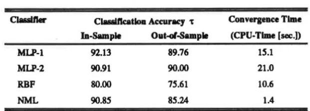
The purpose of the first experiment is to compare the in-sample and out-of-sample performance of

the three neural classifiers each with 196 parameters, where the degrees of freedom are equal to 14.

Thus, we were able to analyse the effect of different hidden unit activation functions, the sigmoid

(logistic), the hyperbolic tangent (tanh) and the radial basis activations, upon performance. All

other factors including initial conditions are fixed in these simulations (rt=0.8). The results are

outlined in table 2 and show that the two MLP-classifiers trained more slowly than the

RBF-classifier, but clearly outperform RBF (measured in terms of 't). The RBF-classifier does not train

and generalize as accurately as the MLP-networks. Its results, however, strongly depend on the

have been made here to optimise the results of this classifier with respect to these parameters. There

seems to be much unexplored potential to improve the performance of this classifier. MLP-1 and

MLP-2 generally train and generalize at the same rate, but MLP-1 'straining is faster, by about 30

percent.

Table 2: Summary ol Classification Results

MLP-1

MLP-2

RBF

NML

Clalalftcatloa Accuracy 't

In-Sample Out-of-Sample

92.13 89.76

90.91 90.00

80.00

90.8S

7S.61

8S.24

Convergence Time

(CPU-Time [sec.])

lS.l

21.0

10.6

1.4

Thus, the best overall result is provided by the MLP-1 classifier with 14 hidden units and 196 free

parameters, followed by MLP-2, and RBF. Both MLP classifiers outperform the NML classifier in

terms of generalization capabilities. The superiority of the MLP classifiers over RBF may be,

moreover, underlined by considering the in-sample and out-of-sample classification error matrices

(see appendix B), the map user's and map producer's accuracies in appendix C. Even though

trained on 1,640 pixels only, the MLP-1 classifier can be used to classify the 97,200 pixels of the whole image. The raw satellite image and the MLP-1 classified image are displayed in figure 4.

4.2 Stability with Training Time

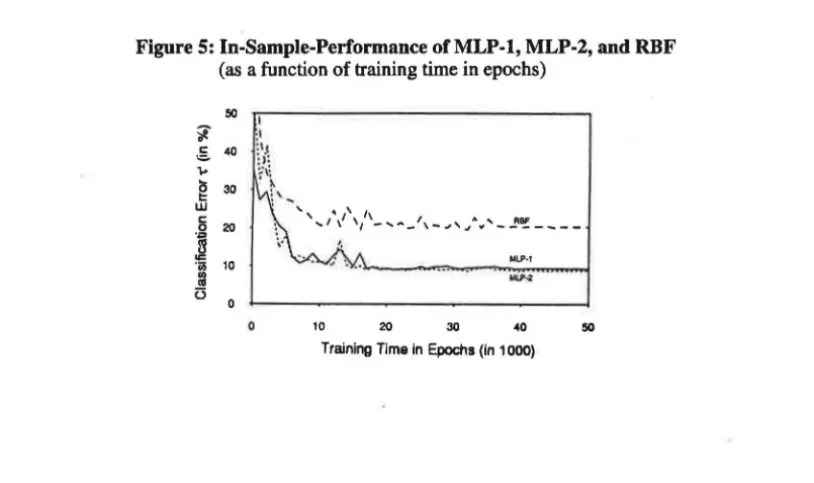
Figure 5 shows the in-sample performance for the two versions of the multi-level perceptron,

MLP-1 and MLP-2, and the radial basis function classifier as a function of training time in epochs

(11=0.8, trained for 50,000 epochs, and equal random initialisations). The in-sample performance tends to converge asymptotically at a minimum that is found at about 17 ,000 epochs in the case of

the MLP-classifiers and about 36,000 epochs in the case of RFB.

There are some regions with temporary performance drops. At least, in the case of the

MLP-classifiers we do not think that these can be interpreted as signs of overtraining, because they

appear rather early in the training process. More probably, their existence implies that the network

is still undertrained, and the better solutions are yet to come for larger numbers of epochs. This

Figure 5: In-Sample-Performance ofMLP-1, MLP-2, and RBF (as a function of training time in epochs)

50

it

c 40

=

..

30

t:: w

6 20

]

·0 10

::!

u

0

0

I ·I

h1

:i:

~~

' ~

: '-...

' ' " _{.... 1 \} 1' _{'1 _ , ... _1, _} ,,

_,,_,"",,'-1'~----Mll'·1

10 20 30 40

Training Time in Epochs (in 1000)

4.3 Stability with Initial Conditions

Backpropagation is known to be sensitive to the values of initial conditions of the parameters. The

number of free parameters of MLP- 1 is 196. The objective function has multiple local minima and is sensitive to details of initial values. A relatively small change in the initial values for the

parameters generally results in finding a different local minimum. In this type of experiment we

used three different sets of initial conditions. Initial weights were chosen from a uniform random distribution in (-0.1, +0.1 ).

Figure 6: The Effect of Different Initial Parameter Conditions on the Performance ofMLP-1

50

..§.. 40

...

g

w

5 20

~

·o; 10

l3

C3

(a) In-Sample Performance

0 10 20 30 40 50

Training Time in Epochs (in 1000)

50 "i

§. 40

...

g

w

c

0

20

...

rl

..,

·o;

10

l3

u

0

.

(b) Out-of-Sample Performance

0 10 20 30 40

Figure 6 shows the in-sample and out-of-sample classification error curves for the three trials. It is

clear, that different initial conditions can lead to more or less major differences in the starting stage

of the training process. After about 15,000 epochs the differences in performance more or less

vanish. Nevertheless, it is important to stress that the issue of stability with initial conditions

deserves consideration when training a classifier in a real-world application context.

4.4 Stability with the Gradient Descent Control Term Tl

The choice of the control parameter for the gradient descent along the surface essentially influences

the magnitude of weight changes and, thus, is crucial for learning performance. But it is difficult to

find appropriate learning rates. On one hand, a small learning rate implies small changes even

though greater weight changes would be necessary. On the other hand, a greater learning rate

implies greater weight changes. Greater weight changes might be required because of the speed of

convergence on the network stability. Larger learning rate values might also assist the classifier to

escape from a local minimum.

It is important to examine how the classification results vary with the gradient descent control term.

A stability analysis with respect to this parameter shows that both in-sample and out-of-sample

performance of the classifier remain very stable in the range of 11=0.4 to 11=0.8, while a small

change from 11=0.4 to 11=0.2 yields a dramatic loss in classification accuracy (see table 3). The

optimal learning rate is the one which has the largest value that does not lead to oscillation, and this

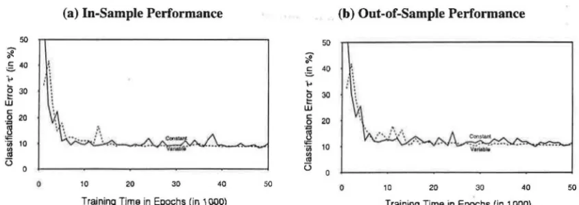
is 11=0.8 in this experiment. Figure 7 shows that a variable learning rate adjustment (declining

learning rate: 11=0.8 until 5,000 epochs, 11=0.4 until 15,000 epochs, then 11=0. l until 35,000 epochs and thereafter Tl =0.00625) might lead to faster convergence, but only to a slightly better

generalization performance.

Figure 7: The Effect of Different Approaches to Learning Rate Adjustment on (a) In-Sample Performance and (b) Out-of-Sample Performance of MLP-1: Constant ('fl=0.8) Versus Variable Learning Rate Adjustment

(a) In-Sample Performance (b) Out-of-Sample Performance

50 ₅₀

~

c: 40

<::.

...

C5 30

I: w

c: 20

0

,,,

:'l "" 10

.iii

"'

"'

0

0 10 20 30 40 50 _{0 10 20 30 40 50}

Table 3: Stability of Results with the Gradient Descent Control Parameter as Function of Training Time in Epochs

Epochs Control Parameter In-Sample Performance Out-of-Sample Performance

(x 103)

11 (in terms of 't) (in terms of 't)

3 0.2 16.6 12.5

0.4 73.7 72.3

0.6 78.2 78.5

0.8 82.2 78.5

6 0.2 17.60 12.5

0.4 90.17 88.2

0.6 86.93 86.0

0.8 88.28 84.9

9 0.2 21.56 12.5

0.4 89.37 88.2

0.6 90.22 87.5

0.8 89.97 87.6

12 0.2 21.56 12.5

0.4 88.37 85.4

0.6 88.38 86.5

0.8 90.92 86.8

15 0.2 22.54 12.7

0.4 90.06 89.1

0.6 88.93 87.9

0.8 89.86 87.3

18 0.2 24.50 13.1

0.4 89.55 87.3

0.6 89.96 87.1

0.8 90.51 88.5

21 0.2 24.50 13.1

0.4 90.77 87.7

0.6 91.48 88.3

0.8 90.22 86.6

24 0.2 31.51 15.4

0.4 91.47 88.2

0.6 90.69 88.0

0.8 87.87 84.3

27 0.2 31.51 15.4

0.4 91.11 89.0

0.6 89.96 87.2

0.8 88.95 88.2

30 0.2 31.51 15.4

0.4 90.81 89.2

0.6 90.29 87 .9

0.8 90.59 87.5

4.5. Stability of Results with Different Training and Testing Samples

All the simulations we mentioned so far were performed for the same training and test data sets,

obtained by stratified random sampling. To examine the effect of different training and test data

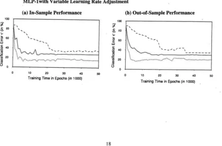
training and testing sets of 1,640 and 820 pixels, respectively. In figure 8 we see only minor

differences. The in-sample performance of the. classifier did not alter significantly after 15,000

epochs. The out-of-sample performance of two trials was rather similar after 36,000 epochs.

However, one of the trials shows a different pattern in out-of-sample performance. If the training

and test samples were randomly drawn without stratification, major differences in performance

might arise between the trials (see figure 9 ).

Figure 8: The Effect of Selected Randomly Chosen Training/Testing Set Trials with Stratification on (a) In-Sample Performance and (b) Out-of-Sample Performance of MLP-lwith Variable Learning Rate Adjustment

50

~40

=

0

(a) In-Sample Performance

. :-._ - - - -J··-- -

r .. _

---10 20 30 40

Training Time in Epochs (in 1 000)

50

~

§.40

..

g

g

fl

""

'ill 10

rd (3

0 50

(b) Out-of-Sample Performance

,...; •,

---0 10 20 30

1,

,,

I

40

Training Time in Epochs (in 1 000)

50

Figure 9:The Effect of Selected Randomly Chosen Training/Testing Set Trials without Stratification on (a) In-Sample Performance and (b) Out-of-Sample Performance of MLP-lwith Variable Learning Rate Adjustment

100

~

~ 60

..

(5

~ 60

c

4D 0

~

·;;; l3

(3

0 0

\

~. ··.

(a) In-Sample Performance

... ' \

-... _...

_

I

....

_____

__

__ _

. ·

...

10 20 30 40

Training Time in Epochs (in 1000)

50

100

~

§. 80

..

60

I:

w

c

0 40 .,.

fl

-=

·0 20 "'

OS

(3 0

(b) Out-of-Sample Performance

'

0

-- ,

10 I

I _....

__

20 30 40

Training Time in Epochs (in 1000)

5. Conclusions

One major objective of this paper was to evaluate the classification accuracy of three neural

classifiers, MLP-1, MLP-2 and RBF, and to analyze their generalisation capability and the stability

of the results. We illustrated that both in-sample and out-of-sample performance depends upon

fine-tuning of control parameters. Moreover, we were able to show that even a simple neural learning

procedure such as the backpropagation algorithm outperforms by about 5 percent the conventional classifier in generalisation that is most often used for multispectral classification on a pixel-by-pixel

basis, the NML classifier. The non-linear properties of the sigmoid (logistic) and the hyperbolic

tangent (tanh) activation functions in combination with softmax activations of the output units

allow neural network based classifiers to discriminate the data better and generalize significantly

better, in the context of this study.

We strongly believe that with careful network design and multiple rather than single training sites

and with a more powerful learning procedure, the performance of the neural network classifiers can

be improved further, especially the RBF classifier. In this respect, other techniques than the

K-means procedure might be more promising to use in order to obtain the initial values for the RBF centres and widths.

We hope that the issues addressed in this paper will be beneficial not only for designing neural

classifiers for multispectral classification on a pixel-by-pixel basis, but also for other classification

problems in the field of remote sensing, such as classification of multi-source data or multi-angle

data.

Acknowledgement

The authors gratefully acknowledge Professor Karl Kraus (Department of Photogrammetric Engineering and Remote Sensing, Vienna Technical University) for his assistance in supplying the remote sensing data used in this study. This work is supported by a grant from the Austrian Fonds zur Forderung der Wissenschaftlichen Forschung (P-09972~

TEC) and the US-National Science Foundation (SBR-930063).

References

Bischof, H., Schneider, W. and Pinz, AJ. (1992): Multispectral classification of Landsat-images using neural networks,

IEEE Transactions on Geoscience and Remote Sensing, vol. 30 (3), pp. 482-490.

Bridle, J.S. (1989): Probabilistic interpretation of feedforward classification network outputs, with relationships to statistical pattern recognition, in Fougelman-Soulie, F. and Herault, J. (eds.): Neuro-Computing: Algorithms, Architectures and Applications, New York: Springer.

Civco, D.L. (1993): Artificial neural networks for land-cover classification and mapping, International Journal of Geographical Information Systems, vol. 7(2), pp. 173-186.

Dreyer, P. (1993): Classification of land cover using optimized neural nets on SPOT data, Photogrammetric Engineering and Remote Sensing, vol. 59(5), pp. 617-621.

Fischer, M.M. and Gopal, S. (1994): Artificial neural networks. a new approach to modelling interregional telecommunication flows, Journal of Regional Science (in press).

Gershenfield, N.A. and Weigend, A.S. (eds.) (1993): Time Series Prediction: Forecasting the Future and Understanding the Past. Reading (MA): Addison-Wesley.

Heerrnan, P.D., and Khazenie, N. (1992): Classification of multispectral remote sensing data using a backpropagation neural network, IEEE Transactions on Geoscience and Remote Sensing, vol. 30(1), pp. 81-88.

Hepner, G.F., Logan, T., Ritter, N. and Bryant, N. (1990): Artificial neural network classification using a minimal training set: Comparison to conventional supervised classification, Photogrammetric Engineering and Remote Sensing, vol. 56 (4), pp. 469-473.

Key, J., Maslanic, A. and Schweiger, AJ. (1989): Classification of merged AVHRR and SMMR Arctic data with neural networks, Photogrammetric Engineering and Remote Sensing, vol. 55(9), pp. 1331-1338.

Lee, J., Weger, R.C., Sengupta, S.K. and Welch, R.M. (1990): A neural network approach to cloud classification, IEEE Transactions on Geoscience and Remote Sensing, vol. 28(5), pp. 846-855.

Refenes, A.N., Zapranis, A. and Francis, G. (1994): Stock performance modeling using neural networks: A comparative study with regression models, Neural Networks, vol. 7(2), pp. 375-388.

Rumelhart, D.E., Hinton, G.E. and Williams, R.J. (1986): Learning internal representation by error propagation, in Rumelhart, D.E., McClelland, J.L. and PDP Research Group (eds.): Parallel Distributed Processing: Explorations in the Microstructures of Cognition, pp. 318-362. Cambridge (MA): MIT Press.

Salu, Y. and Tilton, J. (1993): Classification of multispectral image data by the binary diamond neural network and by nonparametric, pixel-by-pixel methods, IEEE Transactions on Geoscience and Remote Sensing, vol. 31(3), pp. 606-617.

Weigend, AS, Huberman, B.A and Rumelhart, D.E. (1991): Predicting sunspots and exchange rates with connectionist networks, in Eubank, S. and Casdagli, M (eds.): Proceedings of the 1990 NATO Workshop on Nonlinear Modelling and Forecasting, pp. 1-36. Redwood City (CA): Addison-Wesley.

Weigend, AS. (1993): Book Review: John A Hertz, Anders S. Krogh and Richard G. Palmer, Introduction to the Theory of Neural Computation, Artificial Intelligence, vol. 62, pp. 93-111.

White, H. (1989): Some asymptotic results for learning in single hidden-layer feedforward network models, Journal of the American Statistical Association, vol. 84, pp. 1003-1113.

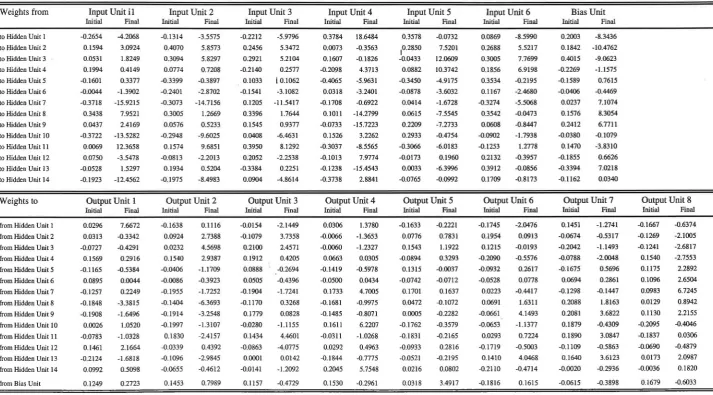
Appendix A: Parameters of the MLP-1 Classifier after Weight Elimination

The classifier was trained for 17,000 epochs with backpropagation and a constant learning rate of 0.8. The connection weights and biases of the network are given below in table Al. When simulated serially on a SPARCserver 10-GS, the training took 15.1 CPU-minutes. Once the parameters have been determined, predictions are extremely fast.

Table Al: Weights of the MNP-1-Classifier after Weight Elimination (17 x 103 epochs)

Weights from

to Hidden Unit I

to Hidden Unit 2

to Hidden Unit 3

to Hidden Unit 4

to Hidden Unit 5

to Hidden Unit 6

to Hidden Unit 7

to Hidden Unit 8

to Hidden Unit 9

to Hidden Unit 10

to Hidden Unit 11

to Hidden Unit 12

to Hidden Unit 13

to Hidden Unit 14

Weights to

from Hidden Unit I

from Hidden Unit 2

from Hidden Unit 3

from Hidden Unit 4

from Hidden Unit 5

from Hidden Unit 6

from Hidden Unit 7

from Hidden Unit 8

from Hidden Unit 9

from Hidden Unit 10

from Hidden Unit 11

from Hidden Unit 12

from Hidden Unit 13

Input Unit il

Initial Final

-0.2654 0.1594 0.0531 0.1994 -0.1601 -0.0044 -0.3718 0.3438 0.0437 -0.3722 0.0069 0.0750 -0.0528 -0.1923 -4.2068 3.0924 1.8249 0.4149 0.3377 -1.3902 -15.9215 7.9521 2.4169 -13.5282 12.3658 -3.5478 1.5297 -12.4562

Output Unit I

Initial Final

0.0296 0.0313 -0.0727 0.1569 -0.1165 0.0895 -0.1257 -0.1848 -0.1908 0.0026 -0.0783 0.1461 -0.2124 7.6672 -0.3342 -0.4291 0.2916 -0.5384 0.0044 0.2249 -3.3815 -1.6496 1.0520 -1.0328 2.1664 -1.6818

Input Unit 2

Initial Final

-0.1314 0.4070 0.3094 0.0774 -0.3399 -0.2401 -0.3073 0.3005 0.0576 -0.2948 0.1574 -0.0813 0.1934 -0.1975 -3.5575 5.8573 5.8297 0.7208 -0.3897 -2.8702 -14.7156 1.2669 0.5233 -9.6025 9.6851 -2.2013 0.5204 -8.4983

Output Unit 2

Initial Final

-0.1638 0.0924 0.0232 0.1540 -0.0406 -0.0086 -0.1955 -0.1404 -0.1914 -0.1997 0.1830 -0.0339 -0.1096 0.1116 2.7388 4.5698 2.9387 -1.1709 -0.3923 -1.7252 -6.3693 -3.2548 -1.3107 -2.4157 0.4392 -2.9845

Input Unit 3

Initial Final

-0.2212 0.2456 0.2921 -0.2140 0.1033 -0.1541 0.1205 0.3396 0.1545 0.0408 0.3950 0.2052 -0.3384 0.0904 -5.9796 5.3472 5.2104 0.2577

I 0.1062

-3.1082 -11.5417 1.7644 0.9377 -6.4631 8.1292 -2.2538 0.2251 -4.8614

Output Unit 3

Initial Final

-0.0154 -0.1079 0.2100 0.1912 0.0888 0.0505 -0.1904 -0.1170 0.1779 -0.0280 0.1434 -0.0863 0.0001 -2.1449 3.7358 2.4571 0.4205 -0.2694 -0.4396 -1.7241 0.3268 0.0828 -1.1155 4.4601 -4.0775 0.0142

Input Unit 4

Initial Final

0.3784 0.0073 0.1607 -0.2098 -0.4065 0.0318 -0.1708 0.1011 -0.0733 0.1526 -0.3037 -0.1013 -0.1238 -0.3738 18.6484 -0.3563 -0.1826 4.3713 -5.9631 -3.2401 -0.6922 -14.2799 -15.7223 3.2262 -8.5565 7.9774 -15.4543 2.8841

Output Unit 4

Initial Final

0.0306 -0.0066 -0.0060 0.0663 -0.1419 -0.0500 0.1733 -0.1681 -0.1485 0.1611 -0.0311 0.0292 -0,1844 1.3780 -1.3653 -1.2327 0.0305 -0.5978 0.0434 4.7005 -0.9975 -0.8071 6.2207 -1.0268 0.4963 -0.7775

Input Unit 5

Initial Final

0.3578 10.2850 -0.0433 0.0882 -0.3450 -0.0878 0.0414 0.0615 0.2209 0.2933 -0.3066 -0.0173 0.0033 -0.0765 -0.0732 7.5201 12.0609 10.3742 -4.9175 -3.6032 -1.6728 -7.5545 -7.2733 -0.4754 -6.0183 0.1960 -6.3996 -0.0992

Output Unit 5

Initial Final

-0.1633 0.0776 0.1543 -0.0894 0.1315 -0.0742 0.1701 0.0472 0.0005 -0.1762 -0.1831 -0.0933 -0.0521 -0.2221 0.7831 1.1922 0.3293 -0.0037 -0.0712 0.1637 -0.1072 -0.2282 -0.3579 -0.2165 0.2816 -0.2195

Input Unit 6

Initial Final

0.0869 0.2688 0.3005 0.1856 0.3534 0.1167 -0.3274 0.3542 0.0608 -0.0902 -0.1253 0.2132 0.3912 0.1709 -8.5990 5.5217 7.7699 6.9198 -0.2195 -2.4680 -5.5068 -0.0473 -0.8447 -1.7938 1.2778 -0.3957 -0.0856 -0.8173

Output Unit 6

Initial Final

-0.1745 0.1954 0.1215 -0.2090 -0.0932 -0.0528 0.0223 0.0691 -0.0661 -0.0653 0.0293 -0.1719 0.1410 -2.0476 0.0913 -0.0193 -0.5576 0.2617 0.0778 -0.4417 1.6311 4.1493 -1.1377 0.7224 -0.5003 4.0468 Bias Unit

Initial Final

0.2003 0.1842 0.4015 -0.2269 -0.1589 -0.0406 0.0237 0.1576 0.2412 -0.0380 0.1470 -0.1855 -0.3394 -0.1162 -8.3436 -10.4762 -9.0623 -1.1575 0.7615 -0.4469 7.1074 8.3054 6.7711 -0.1079 -3.8310 0.6626 7.0218 0.0340

Output Unit 7

Initial Final

0.1451 -0.0674 -0.2042 -0.0788 -0.1675 0.0694 -0.1298 0.2088 0.2081 0.1879 0.1890 -0.1109 0.1640 -1.2741 -0.5317 -1.1493 -2.0048 0.5696 0.2861 -0.1447 1.8163 3.6822 -0.4309 3.0847 -0.5863 3.6123

Output Unit 8

Initial Final

Interpretation of these weights sheds light on which spectral channels are important for particular surface categories. Similarly, the connection weights indicate, for each output category, the degree of information redundancy among channels in the input data. Channels which are only weakly weighted add little additional information to the classification process. The identification of the exact role of the hidden units is difficult, as they often represent generalisations of the input patterns. Figure Al shows with which input data channel each hidden node is associated in the trained network (top) and with which hidden unit each output class is related (bottom). The unit labelled 'bias' has output +1 and so represents the bias term. The areas of the boxes represent the values, the colour the signs (black= positive, white= negative). Following the connections through these two boxes, thus, indicates which input channels are linked to particular output categories.

Figure Al: Weights of the MLP-1-Classifier after Weight Elimination (17 x HP epochs)

Weights lrom Input to Hidden Units Bias

DOD

•••

D

•

D • • •

D D

• • • DD

DD

D

D

~

1

~ 4

•

• D D

DD•D•D•

:>

l

•DD

oo

D•D

a••

oo

D•D

D •

_D

_{• D • o}

4 5 6 7 e 9 10 11 12

Hidden Units

Welglrto to Output lrom Hidden Units

81

D D D

•

•

•

•

a

• •

6

D

•

w

~ 5

l

•

•

3 D

•

•

•

D

•

•

•

D D

D

1 1 . D

•

Hdden Units and Bias

NOie: Thi! •rus or lhe boxes represent the values of lbe weiP,U, the colour the sigm (black= positive, white= negative)

D

•

i-13 14

•

•

•

•

•

D

Appendix B: In-Sample and Out-of-Sample Classification Error Matrices of the Neural Classifiers

An error matrix is a square array of numbers set out in rows and columns which expresses the number of pixels assigned to a particualr category relative to the actual category as verfied by some reference (ground truth) data. The columns represent the reference data, the rows indicate the classification generated. It is important to note that differences between the map classification and reference data might be not only due to classification errors. Other possible sources of errors include errors in interpretation and delineation of the reference data, changes in land cover between the data of the remotely sensed data and the data of the reference data (temporal error), variation in classification of the reference data due to inconsistencies in human interpretation etc.

Classifier's Categories Cl C2 C3 C4 cs C6 C7 C8 Total Classifier's Categories Cl C2 C3 C4 C5 C6 C7 cs

Table Bl: In-Sample Performance: Error Classification Matrices (f1k) of the Neural and the Statistical Classifiers

Cl 157 0 4 0 0 0 0 162 Cl

(a) MLP-1

Ground Truth Categories

C2 C3 C4 CS C6 C7 C8 Total

10

282

0 0

0

0 128

0

0

0 3S9

0 2 0 9 0 0 0 0 0

2 2 9S

0 0 0 0 0 0 0 0 0 0 0 0 0 0 0 10 0

0 0

0 0

0 260 25

0 60 93 0

·o 3 o 104

167 285 128 402 102 296 153 197

292 131 391 109 323 llS 114 1,640

(c) RBF

Ground Truth Categories

C2 C3 C4 CS C6 C7 CS Total

141 22 0

0 4 4 0 0 0 4 O· 0

0 167

14 263 0 2SS

0 0 llS 13 0 0 0 0 128

9 0 0 3 4 9 4 4 0 0 0 402

0 0 12 12 78 0 0 0 102

0 0 5 0 0 1S9 71 31 296

0 0 0 0 0 73 so 0 153

0 0 0 0 0 10 0 97 107

Classifier's Categories Cl C2 C3 C4 C5 C6 C7 C8 Total Classifier's Categories Cl C2 C3 C4 cs C6 C7 cs

Cl C2

1S6 9

4 280

0 4 0 0 0 0 0 0 0 0 0 0

164 289

Cl 161 0 0 0 0 0 0 0 C2 s 284 0 4 0 0 0 0

(b) MLP-2

Ground Truth Categories

C3 0 0 126 C4 2 2

0 384

2 0 0 4 0 0 0 C5 0 0 0 14 96 C6 0 0 0 0 0

0 2S3

0

0 60

4

C7 C8 Total

0 0 0 0 0 2S 0 0 0 0 0 17

93 0

0 103

167 2SS 12S 402 102 296 1S3 107

129 393 110 317 l lS 120 1,640

(d)NML

Ground Truth Categories

C3

0

0

C4

0

124 0

0 3S5

0 0

3 0

0 0

0 0

cs 0 4 13 102 0 0 0 C6 0 0 C7 0 0

CS Total

0

0 167

28S

0 0 0 128

0 0 0 402

0 0 0 102

214 62 17 296

37 116 0 153

Classifier's Categories Cl C2 C3 C4 C5 C6 C1 cs Total Classifier's Categories Cl C2 C3 C4 C5 C6 C1 cs Total Cl 79 0 3 0 0 0 0 S3 Cl 35 5 0 24 0 0 0 0 64

Table B2: Out-of-Sample Error Classification Matrices (f1k) of the Neural and the Statistical Classifiers

(a) MLP-1

Ground Truth Categories

C2 C3 C4 C5 C6 C1

4 134 0 2 3 0 0 0 143

0 0 0 0

6 0 I 0

64 0 0 0

0 194 1 0

0 0 49 0

0 0 0 115

0 0 0 29

0 0 0

70 194 51 145

(c) RBF

Ground Truth Categories 0 0 0 0 0 30 48 0 7S

CS Total

0 S3

0 142

0 64

0 200

0 52

3 14S

0 77

53 54

61 S20

C2 C3 C4 C5 C6 C1 C8 Total

21 137 4 6 26 0 0 0 194 0 0 60 4 4 0 0 0 6S

27 0

0 0

0 0

163 0

0 22

0

0

0

0

0

0 0 104

0 0 29

0 0 0

190 22 133

0 0 0 0 0 35 4S 3 S6

0 S3

0 142

0 64

3 200

0 52

9 14S

0 77

51 54

63 S20

Classifier's Categories Cl C2 C3 C4 C5 C6 C1 cs Total

Classifier' s Categories

Cl C2 C3 C4 C5 C6 C7 cs Total

Cl C2

79 4

140

0 0

2

0

0 0

0 0

0 0

Sl 147

Cl so 0 0 0 0 0 0 Sl C2 3 141 0 3 5 0 0 0 152

(b) MLP-2

Ground Truth Categories

C3 C4 C5 C6

0 0 0 0

0 0 0

64 0 0 0

0 193 3 0

0 0 51 0

0 0 2 110

0 0 0 29

0 0 0

64 193 57 140

(d)NML

Ground Truth Categories

C3 0 0 62 0 0 0 0 63 C4 0 0 0 191 0 0 0 0 191 C5 0 0 5 47 2 0 0 56 C6 0 0 0 0 73 24 2 100 C1 0 0 0 0 0 32 48 0 so C7 0 0 0 0 0 64 53 0 117

CS Total

0 0 0 0 4 0 53 5S S3 142 64 200 52 14S 77 54 S20

C8 Total

Appendix C: In-Sample and Out-of-Sample Map User's and Map Producer's Accuracy

Table Cl: In-Sample C~irlcation Accuracy 7t and u for the Pattern ClaWliers

Category Name Map User's Accuracy 1t Map Producer's Accuracy u

MLP-1 MLP-2 RBF NML MLP-1 MLP-2 RBF NML

Cl Rural Landscape 94.0 93.4 84.4 96.4 96.9 95.1 86.0 95.1

C2 Vineyards 98.9 98.2 92.3 99.6 96.6 96.9 92.3 96.9

C3 Asphalt 100.0 98.4 89.8 96.9 97.7 97.7 87.1 97.7

C4 Woodland 96.8 95.5 86.8 95.8 99.5 97.7 91.4 97.7

C5 Low Residential 96.1 94.1 76.5 100.0 89.9 87.3 63.9 87.3

C6 Densely Built Up 87.8 85.5 63.9 72.3 80.5 79.8 68.5 79.8

C7 Water Courses 60.8 60.8 52.3 75.8 78.8 78.8 53.0 78.8

cs

Table C2: Out-of-Sample C~ilication Accuracy 7t and u for the Pattern Classifiers

Category Name _{Map User's Accuracy 11} Map Producer's Accuracy u

MLP-1 MLP-2 RBF NML MLP-1 MLP-2 RBF NML

Cl Rural Landscape 95.2 95.2 42.2 96.4 95.2 97.5 54.7 98.8

C2 Vineyards 94.4 98.6 96.5 99.3 93.7 95.2 70.6 92.8

C3 Asphalt 100.0 100.0 93.8 96.9 91.4 100.0 88.2 98.4

C4 Woodland 97.0 96.5 81.5 95.5 100.0 100.0 85.8 100.0

.

cs

C6 Densely Built Up 77.7 74.3 70.3 49.3 79.3 78.6 78.2 73.0

C7 W~Courses 62.3 62.3 62.3 68.8 61.5 60.0 55.8 45.3

Manfred M. Fischer is the professor and chair of the Department of Economic Geography at

Wirtschaftsuniversitiit in Vienna. He is the chair of the Commission on Mathematical Models of the

International Geographical Union and is on the Executive Committee of the European Regional

Science Association. He is member of the editorial board of several journals including Environment

and Planning A, Geographical Analysis, The Annals of Regional Science, Papers in Regional

Science and Sistemi Urbani, and he is one of the founding editors of the Geographical Systems,

The International Journal of Geographical Information, Analysis, Theory and Decision. His

research includes geoinformation processing and artificial intelligence, spatial econometrics and

spatial modeling, pattern recognition, decision theory and micro-behavioural modeling. Dr. Fischer

received the MA and Ph.D. degrees in geography and mathematics from the University of

Erlangen, Germany. He was an associate professor at the University of Vienna before assuming his

present position at the Wirtschaftsuniversitiit.

Sucharita Gopal received the Ph.D. in geography from the University of California, Santa Barbara

in 1989. Since then she has carried out research in the area of spatial cognition, fuzzy sets and

spatial accuracy, geographical information systems, and neural network applications. She is an

assistant professor in the Department of Geography at Boston University.

Petra Staufer is an assistant and second year graduate student at the Department of Economic

Geography at Wirtschaftsuniversitiit in Vienna. Her current research interests are irr the field of

neurocomputing, pattern recognition and geographical information systems. She received the MA

degree in geography from the University of Vienna in 1993.

Klaus Steinnocher received the Ph.D. from the Institute of Photogrammetry and Remote Sensing at

the Technical University of Vienna in 1994. He is currently employed at the Department of

Environmental Planning at the Austrian Research Center, Seibersdorf. His research interests

include classification and post classification methods in remote sensing, integration of geographical