Gait based Gender Identification using Statistical
Pattern Classifiers
L.R Sudha
Assistant Professor Department of CSE
Annamalai University Chidambaram
R. Bhavani
Associate Professor Department of CSE Annamalai University Chidambaram
ABSTRACT
Gait based gender identification has received a great attention from researchers in the last decade due to its potential in different applications. This will help a human identification system to focus only on the identified gender related features, which can improve search speed and efficiency of the retrieval system by limiting the subsequent searching space into either a male database or female database. In this paper after preprocessing, four binary moment features and two spatial features are extracted from human silhouette. Then the extracted features are used for training and testing two different pattern classifiers k- Nearest Neighbor (kNN) and Support Vector Machine(SVM). Experimental results show superior performance of our approach to the existing gender classifiers. To evaluate the performance of the proposed algorithm experiments have been conducted on NLPR database.
Keywords
Gender, Gait, Binary moments, Silhouette, Visual Surveillance, kNN, SVM.
1.
INTRODUCTION
Computer Vision Systems are playing more and more important roles in our life with the development of Visual Surveillance and Human Computer Interaction technology. Over past few decades a lot of effort has been devoted in automatic identification of demographic properties such as gender, race and age. Determining the gender of a human is an important visual task that human beings can perform effortlessly from face, voice and through gait. This attracted the attention of Computer Vision and Pattern Recognition community to discover how human brain perceives, represents and remembers these features to identify gender.
Although gender classification has attracted the interest of many, the number of attempts made at automating the process have been fewer in comparison. There are works for classifying gender from voice of the speaker [1], frontal face images and from human walking. In the case of voice, Gender identification can be used before speaker recognition to improve performance by limiting the search space to speakers from same gender. Three main approaches such as using pitch, using Mel Frequency Cepstral Coefficients(MFCC), and combination of knowledge based features and statistical features have been used in voice based gender identification.
Various neural network techniques were employed for gender classification from frontal face image since early 1990’s. Some of the techniques are based on geometric features and others are template based and appearance based. The first attempt was made by Gollomb et al.[2], who trained a
multilayer neural network, SEXNET, to classify gender. Moghaddan and Yang [3] proposed a non-linear SVM for gender classification using the FERET database. Baluja and Rowley [4] presented a method based on Adaboost to identify gender from low_ resolution images. Though human faces provide important visual information for gender perception, in the real world video surveillance systems, it is hard to capture face information at a high enough resolution if the person is far away from the camera.
Compared to face and voice, gait has some unique characteristics. It is a very attractive biometric for real time monitoring and access control at sites of high risk. The suitability of gait in these applications emerge from the fact that gait can be perceived from distance without the consent of the observed object and it cannot be obscured .
Not as many as the ones focused on human identification, but also there have been several studies in gender recognition using gait. Johansson[5], the first researcher attached point-lights to the main joints of the body and film them in a dark background for gender classification and used human observers to classify the gender. But later Troje[6] proposed an automated method instead of human observers. They extract features from point-light displays and presented to a two stage PCA framework for recognizing gender. An adaptive three mode PCA was proposed by Davis and Gao [7] to separate the movements of prototype female and male walkers into posture, time and gender basis sets. They also found that the Correct Classification Rate (CCR) obtained by the human observers are very less when compared with the CCR’s obtained when computer algorithms are used. All the above mentioned studies used point light displays from the aspect of biological motion. But in real time scenarios it is not possible to attach point lights on all objects.
classifier. In [14] shiqi Yu et al. segmented the GEI into five components such as head and hair, chest, back, waist and buttocks, and legs. Then different weights are assigned to different components to form a weighted feature vector
2.
PROPOSED APPROACH
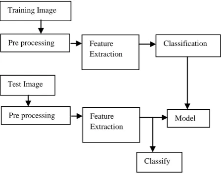
[image:2.595.322.524.101.220.2]In this work we have considered binary silhouettes of frames in two gait cycles of side view videos of normal gait, and extracted six different features. This is because gait of a person is easily recognizable when extracted from side view of a person and majority of the people have normal walk. Our algorithm consists of three main modules namely Preprocessing, Feature Extraction and Classification. Fig.1 gives an overview of the proposed method.
Fig 1: Overview of the Proposed Method
2.1
Preprocessing
Identifying moving objects from a video sequence is a fundamental and critical task in many computer–vision applications. A common approach is to perform background subtraction, which identifies moving objects from the portion of a video frame that differs significantly from a background model. There are many challenges in developing a good background subtraction algorithm
Implementation of this module contains three steps namely background modeling, foreground extraction and binary silhouette generation. First background of the video must be modeled from the frames of the captured video. Many background modeling techniques are available in the literature. But we found that Median value computation is comparatively faster than others. So in our approach we use it to model the background by the equation given below.
)] , ( ) , ( ), , ( [ )
,
(x y medianP1x y P2 x y Pnx y
B (1)
Where P represents a video sequence with N frames and B(x,y) is the background brightness in the pixel location (x,y). After the background is modeled, it is subtracted from the original frames to obtain moving foreground object by the equation given below.
| ) , ( ) , ( | ) ,
(x y P x y B x y
Dk k (2)
In order to be robust to changes of clothing and illumination it is reasonable to consider the binarized silhouette of the object
as in Fig.2. This can be obtained by thresholding the difference image with a suitable threshold value T.
else Foreground
T y x D if Background y
x
Dk k
1
) , ( 0
) ,
( (3)
The assumption made here is that the camera is static, and the only moving object in video sequences is the walker.
Fig 3: i)Whole body ii) Upper body iii) Lower body
2.2
Feature Extraction
In this paper, we have extracted two spatial features and four binary moment features for all the frames in two gait cycles and then calculated the average of each feature for gender discrimination. As shown in Fig.3 features from three different cases of images namely upper body, lower body and whole body are extracted and analyzed
Before the process of feature extraction, we first place a bounding box around the binary silhouette to estimate the gait cycle and thereby to estimate the number of frames in a gait cycle. Knowing the number of frames in a gait cycle, the sequence of binary silhouettes is divided into subsequences of gait cycle length. We then consider frames in two gait cycles for feature extraction. This reduces the processing time considerably. The process of gait cycle estimation is briefly described below.
(a) (b)
Fig. 2 a) Original Image b) Binarized silhouetteModel Pre processing Feature
Extraction Training Image
Test Image
Classify Pre processing Feature
Extraction
[image:2.595.54.279.231.409.2]2.2.1
Gait Cycle Estimation
[image:3.595.319.537.142.410.2]Human gait is treated as a periodic activity within each gait cycle. A single gait cycle, as shown in Fig.4, can be regarded as the time between two identical events during the human walking and usually measured from heel strike to heel strike of one leg. There are two main phases called as stance phase and swing phase in the gait cycle. During stance phase, the foot is on the ground, whereas in swing phase that same foot is no longer in contact with the ground and the leg is swinging through in preparation for the next foot strike. In [15], the aspect ratio of the silhouettes bounding box is used to estimate the gait cycle. In our method width of the bounding box is used as it is periodic and the bounding box will be larger and shorter when the legs are farthest apart and thinner and longer when the legs are together.
Fig 4: Gait cycle of a person
2.2.2
Spatial Feature Computation
Bounding rectangle’s mean height ‘h’ is the representative height value for a person [16]. It is obtained by averaging the difference between upper and bottom points on y axis at each time instant t given by
N t Y t Y h
N
i
i bp up
1
)] ( ) ( [
(4)
where Yup is the upper point on y axis, Ybp is the bottom point
on y axis and N is the number of frames in the gait cycle.
Similarly bounding rectangle’s mean width W is the representative width value of a person. It is obtained by averaging the difference between right and left points on axis x at each time instant t given by
N t X t X W
N
i
i lp rp
1
)] ( ) ( [
(5)
where Xrp is the right point on x axis, Xlp is the left point on x
axis and N is the number of frames in the gait cycle.
2.2.3
Binary Moment Feature Computation
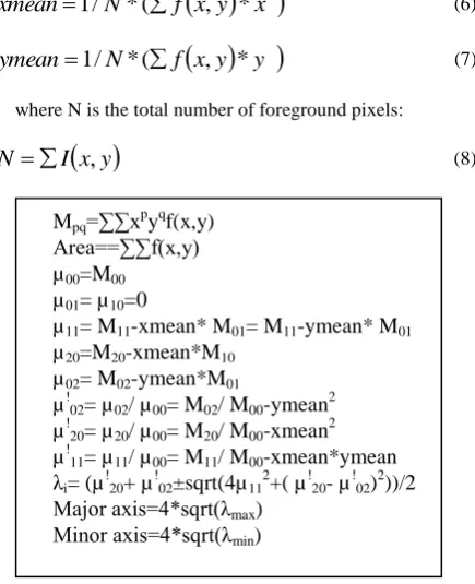
The various binary image properties are given as 0th, 1st and 2nd order moments. The area is given by 0th moment of object. The centroid is given by 1st order moments as (M10, M01) and
2nd order moments give the orientation of the object with the axis.
Let f(x, y) be the binary image in which we want to fit an ellipse. Assume that the foreground pixels are 1 and the background pixels are 0 then the mean x and y of the foreground pixels or the centroid of the region is given by the following equations.
x
y
x
f
N
xmean
1
/
*
(
,
*
(6)
x
y
y
f
N
ymean
1
/
*
(
,
*
(7)where N is the total number of foreground pixels:
x
y
I
N
,
(8)Fig 5: Binary moments of an image
Fig.5 gives the formulas for different binary moments. From the binary moments the aspect ratio ‘l’ and angle of orientation ‘α’ are given as follows.
axis
axis/minor
major
ratio
Aspect
(9)
2 '11/ '20 '02
tan5 .
0
a
Angle (10)
As mentioned above two spatial features and four binary features are extracted from each frame of a walking sequence and averaged to get the feature vector given below.
r
ih
iw
ix
iy
il
i i
f
,
,
,
,
,
(11)3.
EXPERIMENTAL RESULTS
Gender Classification is a traditional pattern classification problem which can be solved by calculating the similarities between instances in the training database and test database. In this work kNN and SVM models are used to find gender of a person and the models are explained in the following subsections. To evaluate performance of the proposed algorithm, experiments are conducted with NLPR database.
3.1
SVM Classifier
Recently, Support Vector Machines (SVM), proposed by Cortes and Vapnik in 1995 has emerged as a powerful supervised learning tool for general purpose pattern recognition. It has been applied to classification and
Mpq=∑∑x p
yqf(x,y) Area==∑∑f(x,y) µ00=M00
µ01= µ10=0
µ11= M11-xmean* M01= M11-ymean* M01
µ20=M20-xmean*M10
µ02= M02-ymean*M01
µ!02= µ02/ µ00= M02/ M00-ymean 2
µ!20= µ20/ µ00= M20/ M00-xmean
2
µ!11= µ11/ µ00= M11/ M00-xmean*ymean
λi= (µ !
20+ µ !
02±sqrt(4µ11 2
+( µ!20- µ !
02) 2
))/2 Major axis=4*sqrt(λmax)
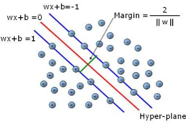
[image:3.595.56.291.238.397.2]regression problems with exceptionally good performance on a range of binary classification tasks [17]. In SVM the original input space is mapped into a high dimensional dot product space called feature space, and in the feature space the optimal hyper plane as shown in Fig. 6 is determined to maximize the generalization ability of the classifier. The primary advantage of SVM is its ability to minimize both structural and empirical risk leading to better generalization for new data classification even when the dimension of input data is high with limited training dataset. SVM can be trained both as a binary classifier and multi-class classifier.
Fig 6: Support Vector Machine
To produce a SVM classifier for class C, the SVM must be given a set of training data including positive and negative samples. Positive samples belong to one class and negative samples belong to other. SVM will find a separating hyper-plane with maximum margin to separate positive and negative examples from the training data
3.2
kNN Classifier
kNN is a method for classifying objects based on closest training examples in the feature space. It is the simplest of all algorithms for predicting the class of a test example. This algorithm contains following three steps to classify objects.
1) Calculate distances of all training vectors to test vector.
2) Pick k closest vectors.
3) Calculate average/majority.
If k = 1, then the object is simply assigned to the class of its nearest neighbor. The best choice of k depends upon the data; generally, larger values of k reduce the effect of noise on the classification, but make boundaries between classes less distinct. A good k can be selected by various heuristic techniques, for example, cross validation. The special case where the class is predicted to be the class of the closest training sample (i.e. when k = 1) is called the nearest neighbor algorithm. To calculate distances of all training vectors to test vector, distance measures such as Euclidean distance, Cityblock distance, Cosine distance, Correlation, Hamming distance can be used. The most common distance function is Euclidean distance. The accuracy of the k-NN algorithm can be severely degraded by the presence of noisy or irrelevant features, or if the feature scales are not consistent with their importance.
The training phase is trivial: simply store every training example, with its label. To make a prediction for a test example, first compute its distance to every training example.
Then, keep the k closest training examples. Look for the label that is most common among these examples. This label is the prediction for this test example. There are two major design choices to make: the value of k, and the distance function to use. When there are two alternative classes, in order to avoid ties the most common choice for k is a small odd integer, for example k = 3. If there are more than two classes, then ties are possible even when k is odd. Ties can also arise when two distance values are the same. An implementation of kNN needs a sensible algorithm to break ties there is no consensus on the best way to do this.
3.3
Classification Results and Analysis
For each lateral view videos of NLPR gait database, we first generate silhouette images using background subtraction algorithm and then silhouette image features are extracted as explained in above section. Then we trained two classification models SVM and KNN with the 6 features and the genders are classified by the trained models at last. We report results in terms of cumulative match scores. To calculate these scores, we conduct multiple tests using multiple test sequences. Each test sequence is compared to the sequences in the reference database.
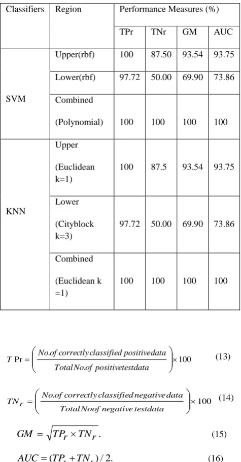
In SVM, experiments were conducted with various kernel types such as linear, Polynomial, and Radial basis function kernels. When compared the results, we found that SVM with Radial Basis Function performs best in both upper and lower region. When the silhouette is considered as a single region, Polynomial kernel gives best performance. The results for these tests conditions are reported in Table 1.
In KNN, experiments were conducted with various distance measures such as Euclidean, Cityblock, Cosine and Correlation and for various K=1 and K=3. We found that classification performance of KNN depends on the selection of K value and distance measure. So it has to be carefully selected to achieve maximum classification accuracy. For gender classification Euclidean distance and City Block distance with K = 1 shows best performance for the upper region and combined region. For the lower part City Block distance with K= 3 gives best performance. All these results are tabulated in Table 2.
Table 1. Performance Comparison of Upper, Lower and Whole body Region using SVM Classifier
Kernel Types Performance Rate (%)
Upper body
Lower body
Whole body
Linear 95.83 87.5 93.75
Polynomial 95.83 83.33 100
Radial Basis Function (RBF)
[image:4.595.342.549.580.718.2]Table 2. Performance Comparison of Upper, Lower and Whole body Region using kNN Classifier
The precision rate of SVM and KNN models are summarized in Table 3, from which it can be seen that SVM and kNN gives 100% performance for whole body silhouette image. Precision rate of the classifiers are calculated using eq.(12). The experiments for the proposed approach were conducted on a personal computer with an Intel Core 2 Duo processor (2.19 GHz) and 1 GB RAM configured with Microsoft Windows XP and Matlab software with image processing toolbox and bio informatics toolbox.
100 .
.
Pr
testdata of No Total
testdata classified correctly
of No
ecision
(
12)
Table 3.Classification rates of different classifiers
[image:5.595.310.548.186.642.2]In this work apart from Precision rate, other measures such as True Positive rate(TPr), True Negative rate(TNr), Geometric mean(GM) and Area Under Classification result(AUC) which are more appropriate for imbalanced problems are also considered and the values are tabulated in Table 4. The formulas for the above performance measures are given below.
Table 4. Comparison of different performance measures
100 .
.
Pr
testdata positive of No Total
data positive classified correctly of No
T
(13)
100 .
testdata negative of No Total
data negative classified correctly
of No r
TN
(14)
.
r
TN
r
TP
GM
(15). 2 / ) (TPr TNr
AUC (16)
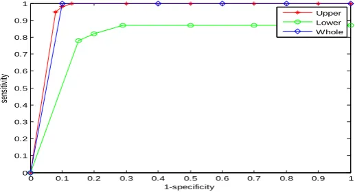
Fig.7 shows the ROC curves for different regions of the silhouette using SVM and kNN Classifier.
Region Distance
Measures
Precision Rate(%)
K = 1 K = 3
Upper body
Euclidean 97.91 87.5
City Block 97.91 91.66
Cosine 79.16 89.58
Correlation 79.16 83.33
Lower body
Euclidean 77.08 87.50
City Block 72.91 89.58
Cosine 75.00 50.00
Correlation 50.00 50.00
Whole body
Euclidean 100 94.23
City Block 100 90.38
Cosine 86.53 86.53
Correlation 82.69 86.53
Classifier Type Precision Rate(%)
kNN 100
SVM 100
Classifiers Region Performance Measures (%)
TPr TNr GM AUC
SVM
Upper(rbf) 100 87.50 93.54 93.75
Lower(rbf) 97.72 50.00 69.90 73.86
Combined
(Polynomial) 100 100 100 100
KNN
Upper
(Euclidean k=1)
100 87.5 93.54 93.75
Lower
(Cityblock k=3)
97.72 50.00 69.90 73.86
Combined
(Euclidean k =1)
[image:5.595.47.234.625.694.2]4.
CONCLUSION
This paper presented a gait based gender identification system using pattern classifiers such as kNN and SVM. These classifiers are employed on NLPR database to evaluate the performance of our approach. We have used only six features to identify gender and got 100% precision rate. This shows the discriminatory ability of the extracted features. This view and appearance dependent model of gait can be further extended to accommodate a multiple appearance model of a person and in conjunction with other recognition modalities.
5.
REFERENCES
[1] H.Harb and L.Chen, 2003. Gender identification using a general audio classifier, In Proc. Int. Conf. Multimedia and Expo, Washington.
[2] B.A Golomb, D.T Lawrence and T.J Sejnowski, 1991. Sexnet:A neural network identifies sex from human faces, Advances in Neural Information Processing Systems.
[3] B. Moghadaam and M.H Yang, 2000. Sex with Support Vector Machines, in NIPS.
[4] S. Baluja and H.A Rowleey, 2007. Boosting sex identification performance, Int. J. Comput. Vision.
[5] G. Johansson, 1973. Visual perception of biological motion and a model for its analysis, Perceptron and Psycophysics.
[6] N.F Troje, 2002. Decomposing biological motion a framework for analysis and synthesis of human gait patterns, J. Vision.
[7] J.W Davis and H.Gao, 2004. Gender recognition from walking movements using adaptive three mode PCA, in Proc. Conf. Computer Vision and Pattern Recognition workshop, Washington.
[8] L.Lee,2003. Gait analysis for classification, Technical report, MIT AI Lab.
[9] L.Lee, W.E.L Grimson, 2002. Gait analysis for recognition and classification in IEEE International Conference on Automatic Face and Gesture Recognition.
[10] X.Li, S.J Maybank, D. Tao, 2007. Gender recognition based on local body motions in IEEE International Conference on Systems, Man and Cybernetics.
[11] X.Li, S.J Maybank, S.Yan, D.Tao, D.Xu, 2008. Gait Components and their applications to gender recognition, IEEE Trans. Syst. Man. Cybern. Part.
[12] L.Cao, M.Dikman, Y.Fu and T.S Huang, 2008. Gender recognition from body, in Proc. 16th ACM Int. Conf. Multimedia.
[13] N.Dalal and B.Triggs,2005. Histograms of oriented gradients for human detection, in Proc. IEEE Conf. ComputeVision and Pattern Recognition.
[14] Shiqi Yu, Tieniu Tan, Kaiqi Huang, Kui Jia and Xinyu Wu, 2009. A study on Gait-Based Gender Classification, IEEE Trans. On Image Processing.
[15] L.Wang, T.Tan, H.Ning and W.Hu, 2003. Silhouette analysis based gait recognition for human identification, IEEE transactions on Pattern Analysis and MachineIntelligence.
[16] Edward Guillen, Daniel Padilla, Adriana Hernandez, Kenneth Barner, 2009. Gait Recognition System: Bundle Rectangle Approach, World Academy of Science, Engineering and Technology.
[17] Rezaul K. Begg, Marimuthu Palaniswami, Brendan Owen , 2005. Support Vector Machines for Automated Gait Classification, IEEE transactions on Biomedical Engineering.
0 0.1 0.2 0.3 0.4 0.5 0.6 0.7 0.8 0.9 1 0
0.1 0.2 0.3 0.4 0.5 0.6 0.7 0.8 0.9 1
1-specificity
se
ns
iti
vi
ty
[image:6.595.164.423.474.614.2]Upper Lower Whole