On a System of Second Order Nonlinear Difference Equations

(1)

http://dx.doi.org/10.4236/jamp.2015.37110

On a System of Second-Order Nonlinear

Difference Equations

Hongmei Bao

Faculty of Mathematics and Physics, Huaiyin Institute of Technology, Huai’an, China Email: [email protected]

Received 29 June 2015; accepted 24 July 2015; published 27 July 2015

This work is licensed under the Creative Commons Attribution International License (CC BY). http://creativecommons.org/licenses/by/4.0/

Abstract

This paper is concerned with dynamics of the solution to the system of two second-order nonli-near difference equations 1

1 1

n n

x

x A

x y

+

− −

= + , 1

1 1

n n

y

y A

x y

+

− −

= + , n= 0,1,, where A∈

(

0,∞

)

,

(

0,

)

i

x₋ ∈ ∞ , y₋_i∈

(

0,∞

)

, i = 0, 1. Moreover, the rate of convergence of a solution that converges to

the equilibrium of the system is discussed. Finally, some numerical examples are considered to show the results obtained.

Keywords

Difference Equation, Boundedness, Stability, Rate of Convergence

1. Introduction

(2)

been published quite a lot of works concerning the behavior of positive solutions of systems of difference equa-tions [1]-[8]. These results are not only valuable in their own right, but they can provide insight into their diffe-rential counterparts.

Papaschinopoulos et al. [1] investigated the global behavior for a system of the following two nonlinear dif-ference equations.

1 , 1 , 0,1, ,

n n

n p n q

y x

x A y A n

x y

+ +

− −

= + = + = 

where A is a positive real number; p and q are positive integers, and x₋_p,,x y₀, ₋_q,,y₀ are positive real numbers.

Clark and Kulenovic [2] [3] investigated the system of rational difference equations.

1 , 1 , 0,1, ,

n n

x y

x y n

a cy b dx

+ = ₊ + = ₊ = 

where a b c d, , , ∈

(

0,∞

)

and the initial conditions x₀ and y₀ are arbitrary nonnegative numbers. Yang [4] studied the system of high-order difference equations.

1 _, 1 _, _{1, 2,}

n n

n p n q n r n s

y x

x A y A n

x y x y

− −

− − − −

= + = + = 

where p≥2,q≥2,r≥2,s≥2,A∈

(

0,+∞

)

, and initial values x_{1 max}₋ _{{ }}_{p r}_, ,x_{2 max}₋ _{{ }}_{p r}_, ,,x y₀, _{1 max}₋ _{{ }}_{q s}_, ,

{ } 0 2 maxq s, , ,

y₋  y are positive real numbers.

Zhang, Yang and Liu [5] investigated the global behavior for a system of the following third order nonlinear difference equations.

2 2

1 1

2 1 2 1

, ,

n n

n n n n n n

x y

B y y y A x x x

− −

+ +

− − − −

= =

+ +

where A B, ∈

(

0,∞

)

, and initial values x₋_i,y₋_i∈

(

0,∞

)

,i=0,1, 2.

Zhang, Liu and Luo [6] studied dynamical behavior for third-order system of difference equations

1 1

1 2 1 2

, ,

n n

n n n n

x y

x A y A

y y x x

+ +

− − − −

= + = +

where A∈

(

0,+∞

)

, and initial values x₋₂,x₋₁,x y₀, ₋₂,y₋₁,y₀ are positive real numbers.

Ibrahim [7] has obtained the positive solution of the difference equation system in the modeling competitive populations.

1 1

, .

n n

n n n n

x y

x y α y x β

− −

+ +

− −

= =

+ +

Din et al. [8] studied the global behavior of positive solution to the fourth-order rational difference equations

3 1 3

1 1

1 2 3 1 1 1 2 3

,

n n

n n n n n n n n

x y

y y y y x x x x

α α

β γ − β γ −

+ +

− − − − − −

= =

+ +

where the parameters α β γ α β γ, , , ₁, ₁, ₁ and the initial conditions x−i,y−i,i=0,1, 2, 3 are positive real numbers. Although difference equations are sometimes very simple in their forms, they are extremely difficult to un-derstand thoroughly the behavior of their solutions. In book [9], Kocic and Ladas have studied global behavior of nonlinear difference equations of higher order. Similar nonlinear systems of difference equations were inves-tigated (see [10]-[19]).

Our aim in this paper is to investigate the solutions, stability character and asymptotic behavior of the system of difference equations

1 1

1 1 1 1

, , 0,1, ,

n n

n n n n

x y

x A y A n

x y x y

+ +

− − − −

= + = + = _ (1)

(3)

Clearly, if A>0, system (1) has always a positive equilibrium point

( )

2 4 2 4

, , .

2 2

A A A A

c c = + + + + 

 

 

2. Boundedness

Theorem 1. Let

{

(

x yn, n

)

}

be a positive solution of (1), then the following statements holds:

1) xn ≥A y, n ≥A, for each n≥1. 2) If

A

>

1

, then for k≥3, we have

( )

3 3 3 3

2 2

2 2 2 2 2 2

2 2

1 1

, .

1 1 1 1

k k k k

A A A A

x x y y

A A A A

A − A −

   

≤ _ − _+ ≤ _ − _+

− − − −

    (2)

Proof. Assertion 1) is obviously true. Now it only need to prove assertion 2). From (1) and in view of 1), we have, for k≥3, that

1 1

2 2

2 2 2 2

1 1

, .

k k

k k k k

x y

x A A x y A A y

x y A x y A

− −

− − − −

= + ≤ + = + ≤ + (3)

Let u vk, k be the solution of following system, respectively

1 1

2 2

1 1

, .

k k k k

u A u v A v

A − A −

= + = + (4)

such that x₂ =u y₂, ₂ =v₂. We prove by induction that

, , 3.

k k k k

x ≤u y ≤v k≥ (5)

Suppose that (5) is true for k=m≥3. From (3) that it follows that

1 2 2 1 1 2 2 1

1 1 1 1

, .

m m m m m m m m

x A x A u u y A y A v v

A A A A

+ ≤ + ≤ + = + + ≤ + ≤ + = + (6)

Therefore (5) is true. From (4) we have

( )

3 3 3 3

2 2

2 2 2 2 2 2

2 2

1 1

, .

1 1 1 1

k k k k

A A A A

u u v v

A A A A

A − A −

   

≤ _ − _+ ≤ _ − _+

− − − −

    (7)

Then from (3), (5) and (6) the proof of the relation (2) follows immediately.

3. Stability

Theorem 2. Assume that A>2 3, then the unique positive equilibrium point

( )

2 4 2 4

, ,

2 2

A A A A

c c

 ₊ ₊ ₊ ₊ 

 

=_ _

 

is locally asymptotically stable.

Proof. We can obtain easily the linearized system of (1) about the positive equilibrium

( )

c c, is

1 n+ B n

Φ = Φ (8)

where

2 2 2

1

2 2 2

1

0

1 0 0 0

, .

0

0 0 1 0

n

n n

n

x c c c

x

B

y c c c

y − − − − − − − −     − −        

Φ =_ _ _{= } _

− −

 

  _ _

   

(4)

Let λ λ λ λ₁, ₂, ₃, ₄ denote the eigenvalues of matrix B, let D=diag

(

d d d d₁, ₂, ₃, ₄

)

be a diagonal matrix, where

(

)

1 3 1, k 1 2, 4 ,

d =d = d = −kε k= and

2

1 3

0 min , .

4 4

c c

ε  − 

< < _ _  

Clearly, D is invertible. Computing matrix DBD−1, we obtain that

2 2 1 2 1

1 2 1 4

1

1 2 1

2 1 2 2 1

3 2 3 4

1 4 3

0

0 0 0

. 0

0 0 0

c c d d c d d

d d DBD

c d d c c d d d d

− − − − −

− −

− − − − −

−

 − − 

 

=  ₋ ₋ 

 

 

From d₁>d₂ >0 and d₃>d₄>0, it implies that

1 1

2 1 1, 4 3 1.

d d− < d d− <

Furthermore

(

)

2 2 1 2 1 2 1 1 2 2

1 2 1 4 1 2 1 4

1 1 3

1 1 1,

1 2 1 4 1 4

c c d d c d d c d d d d c c

ε ε ε

− ₊ − − ₊ − − ₌ − ₊ − ₊ − ₌ −  ₊ ₊ _< − _<

 ₋ ₋  ₋

 

(

)

2 2 1 2 1 2 1 1 2 2

3 2 3 4 3 2 3 4

1 1 3

1 1 1.

1 2 1 4 1 4

c c d d c d d c d d d d c c

ε ε ε

− ₊ − − ₊ − − ₌ − ₊ − ₊ − ₌ −  ₊ ₊ _< − _<

 ₋ ₋  ₋

 

It is well known that B has the same eigenvalues as DBD−1, we have that

(

) (

)

{

}

1 1 1 2 1 1 2 1 1

2 1 4 3 1 2 1 4 3 2 3 4

1 6

max _i max , , 1 , 1 1.

i

DBD d d d d c d d d d c d d d d

λ − − − − − − − − −

∞

≤ ≤ ≤ = + + + + <

This implies that the equilibrium

( )

c c, of (1) is locally asymptotically stable.

Theorem 3. Assume that

A

>

1

. Then every positive solution of (1) converges to

( )

c c, .

Proof. Let

{

x y_n, _n

}

be an arbitrary positive solution of (1). Let

{

}

{

}

1 lim sup n, n1, , 1 lim inf n, n1, .

n→∞ x x+ λ n→∞ x x+

Λ =  = 

{

}

{

}

2 lim sup n, n1, , 2 lim inf n, n1, .

n→∞ y y+ λ n→∞ y y+

Λ =  = 

From Theorem 2, we have 0< ≤A λ₁≤ Λ < ∞ < ≤₁ , 0 A λ₂≤ Λ < ∞₂ . This and (1) imply that

1 2 1 2

1 2 1 2 1 2 1 2

, , ,

A A λ A λ λ A λ

λ λ λ λ

Λ Λ

Λ ≤ + Λ ≤ + ≥ + ≥ +

Λ Λ Λ Λ

which can derive that

1 2 λ λ1 2.

Λ Λ ≤ (10)

If Λ >₁ λ₁ and Λ >₂ λ₂, this implies that Λ Λ >₁ ₂ λ λ_{1 2}, which contradict to (10). Therefore we have Λ =₁ λ₁ and Λ =₂ λ₂, then the limn→∞xn and limn→∞ yn exist. From the uniqueness of the positive equilibrium

( )

c c,

of (1), we conclude that limn→∞xn=c, limn→∞ yn=c.

Combining Theorem 2 and Theorem 3, we obtain the following theorem.

Theorem 4. Assume that A>2 3. Then the positive equilibrium

( )

c c of , (1) is globally asymptotically stable for all positive solutions.

4. Rate of Convergence

In this section we will determine the rate of convergence of a solution that converges to the equilibrium point

( )

c c, of the system (1). The following result gives the rate of convergence of solution of a system of difference equations

( )

1

n n

(5)

where X_n is a four dimensional vector, A∈C4 4× is a constant matrix, B Z: + →C4 4× is a matrix function satisfying

( )

0, when

B n → n→ ∞ (12)

where ⋅ denotes any matrix norm which is associated with the vector norm.

Theorem 5. [20] Assume that condition (12) hold, if Xn is a solution of (11), then either Xn =0 for all large

n or limn n n X ρ →∞

= (13)

or 1 lim n n n X X ρ + →∞

= (14)

exists and is equal to the moduls of one the eigenvalues of the matrix A.

Assume that limn→∞xn =x, limn→∞ yn=y, we will find a system of limiting equations for the system (1).

The error terms are given as

(

)

(

)

(

)

(

)

1 1 1 0 0 1 1 1 0 0

n i n i i n i

i i

n i n i i n i

i i

x x A x x B y y y y C x x D y y

+ − − = = + − − = =  _{− =} ₋ ₊ ₋    _{− =} ₋ ₊ ₋ 

∑

Set 1 2

,

n n n n

e =x −x e =y −y, therefore it follows that

1 1

1 1 2

1

0 0

1 1

2 1 2

1

0 0

n i n i i n i

i i

n i n i i n i

i i

e A e B e e C e D e

+ − − = = + − − = =  ₌ ₊    ₌ ₊ 

∑

where

(

1

)

(

1

)

0 1 2 0 1 2

1 1 ₁ ₁ ₁ ₁

1

, n n , 0, n n .

n n _n _n _n _n

x y x x

A A B B

x y _x _y _x _y

− −

− − ₋ ₋ ₋ ₋

= = − = = −

(

1

)

(

1

)

0 1 2 0 1 2

1 1

1 1 1 1

1

0, n n , , n n .

n n

n n n n

y y x y

C C D D

x y

x y x y

− −

− − − −

= = − = = −

Now it is clear that

0 0 2 1 1 1 1 2

1 1

lim lim , lim lim lim lim .

n→∞A =n→∞D =_c n→∞A =n→∞B =n→∞C =n→∞D = −_c

Hence, the limiting system of error terms at

( )

0, 0 can be written as

1

n n

E+ =GE (15)

where

(

1 1 2 2

)

T

1 1

, , ,

n n n n n

E = e e₋ e e₋ , and

( )

2 2 2

4 4

2 2 2

1 1 1

0

1 0 0 0

0, 0

1 1 1

0

0 0 1 0

F ij

c c c

G J d

c c c

×  ₋ ₋        = = _{= } _  − −       

(6)

Theorem 6. Assume that A>2 3, and

{

(

x yn, n

)

}

be a positive solution of the system (1). Then, the error

vector

E

_n of every solution of (1) satisfies both of the following asymptotic relations

( )

1

( )

limn 0, 0 , lim n 0, 0

n F F

n n

n

E

E J J

E

λ + λ

→∞ = →∞ =

where λJ_F

( )

0, 0 is equal to the moduls of one the eigenvalues of the Jacobian matrix evaluted at the equili-brium

( )

0, 0 .

5. Numerical Examples

In order to illustrate the results of the previous sections and to support our theoretical discussions, we consider an interesting numerical example in this section.

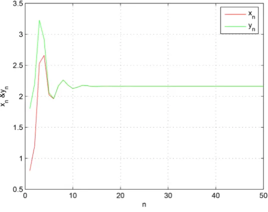
Example 5.1.Consider the system (1) with initial conditions x−₁=0.8,x₀=1.2,y−₁=1.8,y₀=2.2, Moreover,

choosing the parameters A=1.7. Then system (1) can be written as

1 1

1 1 1 1

1.7 n , 1.7 n .

n n

n n n n

x y

x y x y

+ +

− − − −

= + = + (16)

The plot of system (16) is shown in Figure 1.

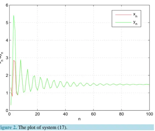
Example 5.2.Consider the system (1) with initial conditions x₋₁=1.3,x₀=0.8,y₋₁=0.3,y₀=1.8, Moreover,

choosing the parameters A=0.8. Then system (1) can be written as

1 1

1 1 1 1

0.8 n , 0.8 n .

n n

n n n n

x x

x y

x y x y

+ +

− − − −

= + = + (17)

The plot of system (17) is shown in Figure 2.

6. Conclusions and Future Work

In this paper, the dynamical behavior of second-order discrete system is studied. It can be concluded that:

1) The positive equilibrium point

2 2

4 4

,

2 2

A A A A

 ₊ ₊ ₊ ₊ 

 

 

[image:6.595.180.448.495.707.2]

is globally asymptotically stable if A>2 3. 2) The equilibrium rate of convergence is discussed. Some numerical examples are provided to support theo-retical results. It is our future work to study the oscillation behavior of system (1).

(7)

[image:7.595.181.454.80.309.2]

Figure 2. The plot of system (17).

Acknowledgements

The author would like to thank the Editor and the anonymous referees for their careful reading and constructive suggestions.

References

[1] Papaschinopoulos, G. and Schinas, C.J. (1998) On a System of Two Nonlinear Difference Equations. Journal of Ma-thematical Analysis and Applications, 219, 415-426. http://dx.doi.org/10.1006/jmaa.1997.5829

[2] Clark, D., Kulenovic, M.R.S. and Selgrade, J.F. (2003) Global Asymptotic Behavior of a Two-Dimensional Difference Equation Modelling Competition. Nonlinear Analysis, 52, 1765-1776.

http://dx.doi.org/10.1016/S0362-546X(02)00294-8

[3] Clark, D. and Kulenovic, M.R.S. (2003) A Coupled System of Rational Difference Equations. Computers and Mathe-matics with Applications, 43, 849-867. http://dx.doi.org/10.1016/S0898-1221(01)00326-1

[4] Yang, X. (2005) On the System of Rational Difference Equations xn= +A yn−1 xn p− yn q− ,yn= +A xn−1 xn r− yn s− . Jour- nal of Mathematical Analysis and Applications, 307, 305-311. http://dx.doi.org/10.1016/j.jmaa.2004.10.045

[5] Zhang, Q., Yang, L. and Liu, J. (2012) Dynamics of a System of Rational Third-Order Difference Equation. Advances in Difference Equations, 136, 1-8. http://dx.doi.org/10.1186/1687-1847-2012-136

[6] Zhang, Q., Liu, J. and Luo, Z. (2015) Dynamical Behavior of a System of Third-Order Rational Difference Equation.

Discrete Dynamics in Nature and Society, 2015, Article ID: 530453. http://dx.doi.org/10.1155/2015/530453

[7] Ibrahim, T.F. (2012) Two-Dimensional Fractional System of Nonlinear Difference Equations in the Modeling Compet-itive Populations. International Journal of Basic & Applied Sciences, 12, 103-121.

[8] Din, Q., Qureshi, M.N. and Khan, A.Q. (2012) Dynamics of a Fourth-Order System of Rational Difference Equations.

Advances in Difference Equations, 2012, 215. http://dx.doi.org/10.1186/1687-1847-2012-215

[9] Kocic, V.L. and Ladas, G. (1993) Global Behavior of Nonlinear Difference Equations of Higher Order with Applica-tion.Kluwer Academic Publishers, Dordrecht. http://dx.doi.org/10.1007/978-94-017-1703-8

[10] Liu, K., Zhao, Z., Li, X. and Li, P. (2011) More on Three-Dimensional Systems of Rational Difference Equations.

Discrete Dynamics in Nature and Society, 2011, Article ID: 178483.

[11] Ibrahim, T.F. and Zhang, Q. (2013) Stability of an Anti-Competitive System of Rational Difference Equations. Arc-hives Des Sciences, 66, 44-58.

[12] Zayed E.M.E. and El-Moneam, M.A. (2011) On the Global Attractivity of Two Nonlinear Difference Equations.

Journal of Mathematical Sciences, 177, 487-499.http://dx.doi.org/10.1007/s10958-011-0474-8

(8)

[14] Touafek, N. and Elsayed, E.M. (2012) On the Solutions of Systems of Rational Difference Equations. Mathematical and Computer Modelling, 55, 1987-1997. http://dx.doi.org/10.1016/j.mcm.2011.11.058

[15] Kalabusic, S., Kulenovic, M.R.S. and Pilav, E. (2011) Dynamics of a Two-Dimensional System of Rational Difference Equations of Leslie-Gower Type. Advances in Difference Equations, 2011, 29.

http://dx.doi.org/10.1186/1687-1847-2011-29

[16] Ibrahim, T.F. (2012) Boundedness and Stability of a Rational Difference Equation with Delay. Revue Roumaine de Mathématiques Pures et Appliquées, 57, 215-224.

[17] Ibrahim, T.F. and Touafek, N. (2013) On a Third-Order Rational Difference Equation with Variable Coefficients.

DCDIS Series B: Applications & Algorithms, 20, 251-264.

[18] Ibrahim, T.F. (2013) Oscillation, Non-Oscillation, and Asymptotic Behavior for Third Order Nonlinear Difference Equations. Dynamics of Continuous, Discrete and Impulsive Systems, Series A: Mathematical Analysis, 20, 523-532.

[19] Zhang, Q. and Zhang, W. (2014) On a System of Two High-Order Nonlinear Difference Equations? Advances in Ma-thematical Physics, 2014, Article ID: 729273.