Editors: A. K. Ariffin, N. A. Nik Mohamed and S. Abdullah
SOLUTION TO NAVIER-STOKES EQUATIONS FOR LID-DRIVEN CAVITY PROBLEM: COMPARISONS BETWEEN LATTICE
BOLTZMANN AND SPLITTING METHOD
M. Z. Ngali1, N. A. C. Sidik2, K. Osman2 and A. Z. M. Khudzairi2
1
Faculty of Mechanical and Manufacturing Engineering Universiti Tun Hussein Onn Malaysia
84000 Batu Pahat, Malaysia
2
Faculty of Mechanical Engineering Universiti Teknologi Malaysia 81310 UTM Skudai, Johor, Malaysia
ABSTRACT
Solutions to the Navier Stokes equations have been pursued by many researchers. One of the recent methods is lattice Boltzmann method, which evolves from Lattice Gas Automata, simulates fluid flows by tracking the evolution of the single particle distribution. Another method to solve fluid flow problems is by splitting the Navier Stokes equations into linear and non-linear forms, also known as splitting method. In this study, results from uniform and stretched form of splitting method are compared with results from lattice Boltzmann method. The traditional two dimensional lid driven cavity problems, with constant density, is used as the case study. For low Reynolds number transient problems, the lattice Boltzmann method requires less time as compared to that of splitting method to reach steady state conditions. As the Reynolds number increases, the lattice Boltzmann method begins to consume more time than that of splitting method. However, the lattice Boltzmann method results maintain to be the most accurate when comparisons are made with benchmark results for the same grid configuration.
Keywords: Lattice Boltzmann method; splitting method; lid-driven cavity flow
INTRODUCTION
incompressible flow, one of the most popular velocity-pressure coupling methods is SIMPLE (Semi-Implicit Method for Pressure-Linked Equation).
SIMPLE technique involves major convergence iteration to determine the pressure values for every main velocity-time iteration. As an alternative, (Karniadakis 1991) had introduced a new formulation for high-order time-accurate splitting scheme for the solution of the incompressible Navier-Stokes equations.
Principally, flow problems where large gradients are concentrated in a specific region require refinement of resolutions on those regions. Instead of using uniform, high resolution grid distribution in the physical domain, grid points may be clustered in the regions of high flow gradients and broaden at other regions. Stretched coordinate could demonstrate these advantages with direct usage of mathematical models of Navier-Stokes solution derived in Cartesian coordinate with minimum verifications of the discretization methods.
This work is meant to bring together the advantage of Splitting method as pressure-velocity solver of higher efficiency with the advantage of consuming stretched grid which produce more accurate results in relatively equal number of grid points as compared to Cartesian grid.
Lattice Boltzmann method (LBM), a numerical method based on particle distribution function has been demonstrated to be a very effective numerical tool for a broad variety of complex fluid flow phenomena that are problematic for conventional method (Sidik et. al. 2005). Compared with traditional computational fluid dynamics, LBM algorithms are much easier to be implemented especially in complex geometries and multi-component flows. Historically, LBM was derived from the lattice gas (LG) automata. It utilizes the particle distribution function to describe collective behaviors of fluid molecules. The macroscopic quantities such as density and velocity are then obtained through moment integrations of the distribution function.
MATHEMATICAL METHODS
The temporal integration of the Navier-Stokes system is achieved using a semi-implicit splitting method, similar to the method of (Karniadakis et. al 1991), (Kahar 2004) and others. Consider the Navier-Stokes expression below
(
)
1
L
(
v
),
R
p
v
N
t
v
e
v
v
v
v
v
+
−∇
=
+
∂
∂
(1)
where
L
v
is the linear viscous term andN
v
is the non-linear advective term,. )
(
, )
( 2
v v v N
v v
L
v v v v
v v
v
∇ ⋅ =
∇ =
∫
∫
∫
∫
+ + + ++
∇
−
=
+
∂
∂
1 1 11
,
)
(
1
)
(
k k k k k k k k t t t t t t e tt
t
dt
N
v
dt
pdt
R
L
v
dt
v
v
v
v
v
v
(3)
where k is the time step.
The first term is easily evaluated without approximation. A semi-implicit method treats linear terms implicitly for stability, and non-linear term is achieved with the second-order Adams-Bashforth method. The pressure term is treated by reversing the order of integration and differentiation, then introducing time-averaged pressure while The implicit treatment of the linear viscous term is achieved with the second-order Crank-Nicholson method. The combined difference equation becomes,
[
v v]
tR t p t v N v N v
v k k
e k
k k
k
k ∆ =−∇ ∆ + ∇ +∇ ∆
⎥⎦ ⎤ ⎢⎣ ⎡ − + − − + +
+ v v v v v v v
v 1 1 1 2 1 2
2 1 ) ( 2 1 ) ( 2 3 (4)
The continuity equation is imposed at the leading time step,
.
0
1=
⋅
∇
k+v
v
(5)In splitting method, eq. (4) is integrated numerically in three for each time step, each stage addressing the three terms independently and take divergence of this equation and use the continuity equation to obtain the Poisson’s equation for pressure, , ˆ 1 2 ⎟⎟ ⎠ ⎞ ⎜⎜ ⎝ ⎛ ∆ ⋅ ∇ = ∇ + t v pk v (6)
where the nonlinear term is neglected. Take the normal component of equation 4 to get,
t
v
N
v
N
k
v
k
v
k
p
k
v
⋅
∇
k+1=
v
⋅
v
k−
v
⋅
v
k+1−
v
⋅
⎡
⎢⎣
v
v
k−
v
(
v
k−1)
⎤
⎥⎦
∆
+
2
1
)
(
2
3
k
[
v
v
]
t
R
k k e∆
∇
+
∇
⋅
v
+v
v
2 1 22
1
(7)
(Karniadakis 1991) has shown that all the right hand side terms of above equation can be neglected for large Reynolds number, leaving,
.
0
1=
∇
⋅
k+p
For that reason, (Karniadakis 1991) recommends higher order boundary conditions for a better approximation, especially for low Reynolds number flow.
Regular Cartesian coordinate can be ‘stretched’ according to the specific requirement by the use of algebraic transformation technique. In generating grid coordinate for flow in a duct, (Anderson et. al. 1997) derived a set of algebraic expressions to transform points in computational Cartesian coordinate to physical stretched coordinate and vice versa.
For the case of square cavity flow, algebraic expressions are used to cluster grid points near solid boundaries and critical locations such as the corners of a cavity to provide adequate resolutions for the viscous boundary layer and secondary vortices. Since the transformation for flow in a duct was found to be in a single horizontal direction, modification is done for the cavity flow grid by first transforming the horizontal, x direction and then followed by transforming the vertical, y direction.
The algebraic formulation for transformation between physical and computational domain is shown below:
(
)(
[
) (
)
]
(
) (
)
(
)
{
[
(
) (
)
]
(
η α) (
α)
}
α α η β β α β α β β β α − − − − − + + + − + − + + = 1 1 1 1 1 1 1 1 2 2 1 1 2 Lx (9)
(
)(
[
) (
)
]
(
) (
)
(
)
{
[
(
) (
)
]
(
η α) (
α)
}
α α η β β α β α β β β α − − − − − + + + − + − + + = 1 1 1 1 1 1 1 1 2 2 1 1 2 Hy (10)
For a cavity of width L and height H, where β is the clustering parameter, and
α defines where the clustering takes place. When α = 0 the clustering is at x=L
and y=H; whereas when α =1/2 clustering is distributed equally at the four sides of the cavity. While, the algorithm in LBM generally consists of two steps; collision, which occurs when particle distribution function arrives at a node: and streaming, where the distribution function moves to the nearest nodes in the direction of its velocity. The equation describe these two steps is known as the lattice Boltzmann equation (LBE)
(
+ ∆tt+∆t) ( )
−f t =Ωf x c , x, (11)
where
f
is the distribution function for particles with velocity c at positionx
and time
t
. ∆t is the time increment andΩ
is the collision operator. It was difficult to solve the LBE because the collision term is complicated. One of the most widely used simplified collision model is the BGK collision operator which applies single time relaxation approximation.(
feq−f) (
= feq− f)
=Ω
τ
The coefficient
ω
is called the collision frequency andτ
is called relaxation time. The local equilibrium distribution function denoted byf
eq. In this research, the momentum space is discretised with nine discrete velocities and nine bit model is obtained, i.e., it is discretised into a square lattice space with a uniform lattice. Then the equilibrium distribution function of the nine bit model is(
) (
)
⎪⎭ ⎪ ⎬ ⎫ ⎪⎩ ⎪ ⎨ ⎧ − ⋅ + ⋅ + = 2 2 4 2 2 3 2 9 3 1 c c c wfeq αρ cα u cα u u (13)
The weights are
⎪⎩ ⎪ ⎨ ⎧ = , 36 1 , 9 1 , 9 4 α w
=
=
=
α
α
α
9 , 8 , 7 , 6 5 , 4 , 3 ,2 1 (14)
and
( )
(
)
(
)
⎪⎩ ⎪ ⎨ ⎧ = , sin , cos 2 , sin , cos , 0 , 0 c c α α α α α θ θ θ θ c=
=
=
α
α
α
9 , 8 , 7 , 6 5 , 4 , 3 , 2 1 (15)where θα =
(
α−1)
π 2 for α =2−5,(
α−5)
π 2+π 4 for α =6−9 and c=∆x ∆t. One of the important and crucial issues in lattice Boltzmann simulation of flow is accurate modeling of boundary condition. Boundary conditions in LBM were originally taken from the LG method, known as the bounce back scheme. The easy implementation of this no-slip velocity condition by the bounce back boundary scheme is another advantage of LBM for simulating fluid flows in complicated geometries.The fluid mass density
ρ
, and the fluid velocity u, are defined in terms of the particle distribution function by∑
=
α α
ρ f (16)
∑
=
α α α
ρ c
u 1 f (17)
Through a multiscaling expansion, the mass and momentum equation can be derived for the nine bit model. The detail derivation is given by (Luo et. al. 1997) and will not be shown here.
0 = ⋅
u u
u
u+ ⋅∇ =−1∇ + ∇2
∂
∂ υ
ρ p
t (19)
where
p
=
c
s2 is the pressure, cs = c 3 is the sound speed and the kinematicviscosity is given by
6 1 2 −
= τ
υ (20)
RESULTS
Comparison between all the methods were done by performing computation on traditional driven cavity problem. Results published by Ghia were used as the bench mark for accuracy. Time taken to complete the iterations until steady state conditions were first compared as shown in Figure 1. For 33x33 grid, the shortest time taken to reach steady state condition was shown by LB method, followed by splitting method (Cartesian) and finally by splitting method (stretched).
Although LB method seemed to be very favorable in solving the traditional driven cavity problems, careful attention should be paid to its efficiency in solving them. For higher Re, the vortices and the corners of the domain would be stronger and to predict these eddies, finer grids are needed. Imposing more grids would be more time needed to solve a particular problem. This remark is shown when the number of grid is increased to 65x65. LB method took the longest time to reach steady state condition in all computations. At Re 1000, LB method needed roughly 25 percent more time as compared to that of stretched coordinates. For high Re, the Cartesian coordinate method fails to show acceptable results.
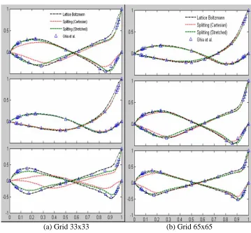
First accuracy comparison was made for grid of 33x33 as in Figure 2(a). For Re = 100. All methods showed good comparison with those of Ghia’s. Looking closely, LB method seemed to agree very well, followed by splitting method using stretched coordinates and finally the least accurate is splitting method using Cartesian coordinates.
FIGURE 1 Efficiency comparison for resolution of 33 x 33 and 65 x 65
[image:7.595.116.475.269.602.2](a) Grid 33x33 (b) Grid 65x65
FIGURE 2 Accuracy comparison for Re 100(top), 400(mid) and 1000(btm)
CONCLUSIONS
Three methods were employed to solve the traditional driven cavity problems with different force strength: Lattice Boltzmann, splitting method with Cartesian coordinates and splitting method with stretched coordinates. For low Re, all methods employed showed good results with relatively coarse mesh. Lattice Boltzmann method also took the shortest time to reach steady state condition. For higher Re, both splitting method with Cartesian coordinates and splitting method with stretched coordinates failed to show results with acceptable accuracy but took shorter time to reach steady state compared to time taken by Lattice Boltzmann method. For the splitting methods, the stretched coordinates results were more accurate compared to those of Cartesian coordinates.
ACKNOWLEDGEMENTS
The author wishes to acknowledge Universiti Teknologi Malaysia and Malaysia Government for supporting this research activity.
REFERENCES
Anderson, D.A., Tannerhill, J.C. & Pletcher, R.H. 1984. Computational Fluid Mechanics and Heat Transfer. 2nd ed., Taylor & Francis.
Ghia, U., Ghia, K. N. &Shin, C.Y., 1982. High-Re solutions for incompressible flow using the Navier-Stokes equations and a multigrid method, J. Comp.Phys. 48: 387-411.
Kahar, O., 2004, Multiple Steady Solutions and Bifurcations in the Symmetric Driven Cavity, Ph. D Thesis, Univerisiti Teknologi Malaysia, Skudai, Johor, Malaysia.
Karniadakis, G., Israeli, K. and Orszag, S., 1991. High-order splitting methods for the incompressible Navier-Stokes equations, J. Comp. Phys. 97: 414-443.