Role of independent component analysis in intelligent ECG signal processing

(1)

ROLE OF INDEPENDENT COMPONENT

ANALYSIS IN INTELLIGENT ECG SIGNAL

PROCESSING

Mohammad Sarfraz

School of Computing, Science and Engineering

University of Salford, Salford, UK

Submitted in Partial Fulfilment of the Requirement of

(2)

i

List of tables

Table ‎7-1 Record and number of ECG sample used ... 85

Table ‎8-1 Comparison of classification Sensitivity before and after source separation. ... 94

Table ‎8-2 Comparison of classification positive predictive value before and after source separation. ... 95

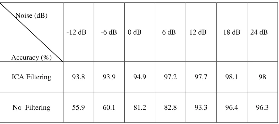
Table ‎8-3 Comparison of classification accuracy before and after source separation. ... 96

Table ‎8-4 Detailed accuracy for different arrhythmias with proposed method ... 104

Table ‎8-5 Detailed positive predictive value for different arrhythmias with proposed method ... 105

Table ‎8-6 Detailed sensitivity for different arrhythmias with the proposed method ... 106

Table ‎8-7 Detailed accuracy for different arrhythmias with SVM classifier ... 108

Table ‎8-8 Detailed positive predictive value for different arrhythmias with SVM classifier 109 Table ‎8-9 Detailed sensitivity for different arrhythmias with SVM classifier... 110

Table ‎8-10 Detailed specificity for different arrhythmias with PCA extracted features ... 112

Table ‎8-11 Detailed sensitivity for different arrhythmias with PCA extracted features... 113

(6)

v

List of figures

Figure ‎3-1 Anatomy of the heart and associated vessels. ... 15

Figure ‎3-2 Electrophysiology of the cardiac muscle cell ... 18

Figure ‎3-3 Basic ECG wave shape with morphological features ... 21

Figure ‎3-4 Einthoven triangle and ECG limb leads definition ... 23

Figure ‎3-5 Augmented lead placement ... 25

Figure ‎3-6 six chest electrodes placement for ECG ... 26

Figure ‎3-7 Different component of ECG during depolarization of atria and ventricle. ... 27

Figure ‎3-8 RBBB arrhythmia recorded by different leads ... 30

Figure ‎3-9 Premature Ventricular Contraction ... 31

Figure ‎4-1 ICA demonstration with Cocktail Party Problem ... 37

Figure ‎4-2 Blind source separation (BSS) block diagram ... 38

Figure ‎4-3 ICA demonstration original source signal ... 39

Figure ‎4-4 ICA demonstration mixed (observed) signal... 40

Figure ‎4-5 ICA demonstration recovered source signal ... 41

Figure ‎4-6 Whitening Process ... 50

Figure ‎4-7 Learning objectives of Infomax ICA algorithm ... 52

Figure ‎4-8 Mixing and de-mixing model ... 53

(7)

vi

Figure ‎6-1 Layout of ANN ... 65

Figure ‎6-2 Three layer back-propagation neural network... 66

Figure ‎6-3 SVM methodology of maximising margin between different classes ... 70

Figure ‎7-1 Proposed setup for removing motion artefacts ... 75

Figure ‎7-2 Motion artefact removal flowchart ... 76

Figure ‎7-3 Sample of „em‟ noise 10 Sec ... 77

Figure ‎7-4 Ambulatory ECG with motion artefact ... 77

Figure ‎7-5 Extracted signal from two leads ... 78

Figure ‎7-6 Original ECG data ... 78

Figure ‎7-7 A normal heartbeat is a linear combination of ICA bases with Coefficients, ... 82

Figure ‎7-8 ECG heartbeats of eight types ... 83

Figure ‎7-9 Block diagram of the proposed feature extraction and classification system ... 86

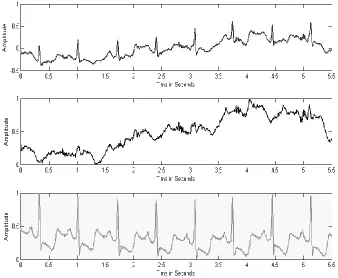
Figure 8-1 ECG Combine with noise (Top Panel), „em‟ Noise middle panel, Extracted ECG with ICA bottom panel. Y Axis is normalized after ICA ... 92

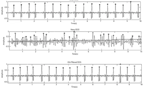
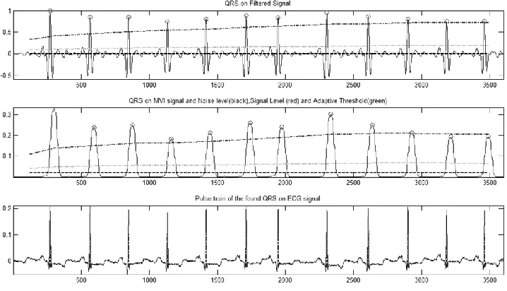
Figure ‎8-2 Pan Tomkins algorithm for beat detection on a sample of a clean ECG, a noisy ECG (SNR= -6 dB) & filtered ECG using ICA. The beat detection has significant improvement after ICA filtering. ... 93

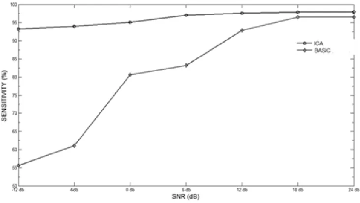
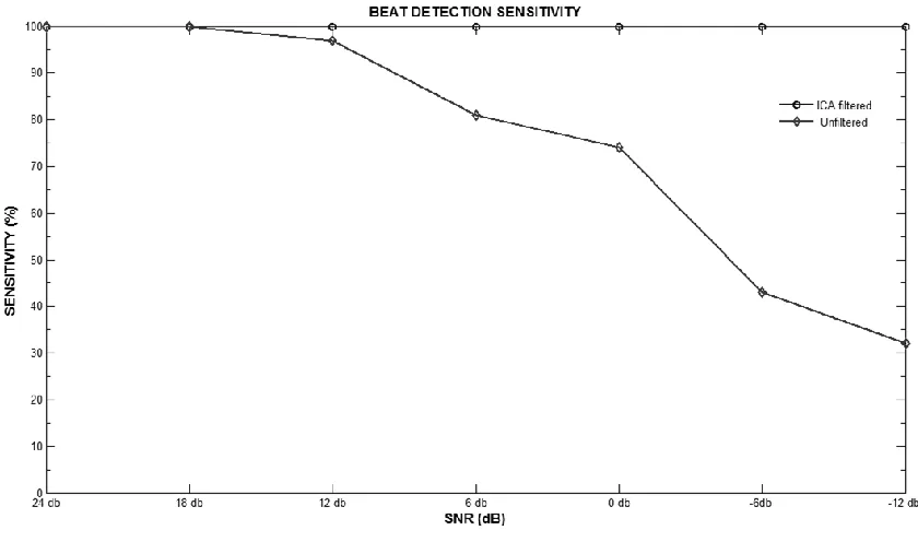
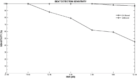
Figure ‎8-3 Sensitivity with ICA filtering and without filtering ... 95

Figure ‎8-4 Positive Predictivity with ICA filtering and without filtering ... 96

(8)

vii

Figure ‎8-6 ECG beat detection using a Pan Tomkins algorithm ... 97

Figure ‎8-7 ECG QRS detection using a Pan Tomkins algorithm ... 98

Figure ‎8-8 Beat detection comparison for LBBB arrhythmia with proposed ICA filtering and without filtering ... 98

Figure ‎8-9 Beat detection comparison for Normal ECG beat with proposed ICA filtering and without filtering ... 99

Figure ‎8-10 Beat detection comparison for RBBB ECG beat with proposed ICA filtering and without filtering ... 99

Figure ‎8-11 Beat detection comparison for VEB arrhythmia with proposed ICA filtering and without filtering ... 100

Figure ‎8-12 Classification into eight classes with proposed method ... 103

Figure ‎8-13 Results of Arrhythmia Classification Accuracy with proposed method ... 104

Figure ‎8-14 Results of positive predictive value with the proposed method ... 105

Figure ‎8-15 Results of sensitivity with the proposed method ... 106

Figure ‎8-16 Results of Arrhythmia Classification Accuracy with SVM classifier ... 107

Figure ‎8-17 Results of positive predictive value with SVM classifier ... 108

Figure ‎8-18 Results of sensitivity with SVM classifier ... 109

Figure ‎8-19 Results of accuracy with PCA extracted features ... 111

Figure ‎8-20 Results of positive predictive value with PCA extracted features ... 111

(9)

(10)

ix

Acknowledgements

I would like to express my sincere gratitude to my supervisor Dr Francis Li for the continuous support of my Ph.D. study and research, for his patience, motivation, enthusiasm, and immense knowledge. His guidance helped me throughout my research and writing of this thesis. Without his invaluable support and encouragement, this thesis would not have been accomplished. He has contributed greatly to every paper I have written, and to every progress I have made.

I would also like to extend my gratitude‟s to Professor P Gaydecki and Professor T Rich ling for their keen interest in my thesis. Their observations are a great source of knowledge as well as realization of some weak areas in my work. I hope their observations will go a long way in my further research endeavours.

My sincere thanks also go to Dr Ateeq Ahmed Khan for being my local supervisor and offering me every support at Salman bin Abdul Aziz University. He has given much help and many suggestions on not only my research and study, but also on my life in Alkharj. I would also like to thank my Dean Dr Osama Saad Alqahtani, College of Engineering, Salman bin Abdul-Aziz University, for his support and motivation for providing me all the help at Salman bin Abdul Aziz University to complete this thesis.

(11)

x

Abbreviations

A Atrial Premature Beat

ANFIS Adaptive Neuro-Fuzzy Inference System

(ANFIS

ANN Artificial Neural Network

ANSI American National Standards Institute

AV Atrio Ventricular

BPNN Back Propagation Neural Network

CVD Cardiovascular Diseases

ECG Electrocardiogram

EEG Electroencephalogram

ERP Event-Related Potentials

F Fusion Of Paced And Normal Beats

GUI Graphical User Interface

HBR Heart Beat Rate

ICA Independent Component Analysis

ISO Isoelectric Line

LMS Least Mean Square

LVQ Linear Vector Quantization

MART Multi-Channel Adaptive Resonance Theory

MIT-BIH Massachusetts Institute Of Technology Beth

Israel Hospital Database

MLP Multi Layer Perceptron

MSE Mean Squared Error

N Normal

NLMS Normalized LMS Algorithms

P Paced Beats

PCA Principal Component Analysis

PPV Positive Predictive Value

PVC Premature Ventricular Contraction

QRS Combination Of 3 Graphical Defection On

(12)

xi

R Right Bundle Branch Block

RBBB Right Bundle Branch Block

RCE Restricted Coulomb Energy

SA Sino Atrial

SNR Signal To Noise Ratio

SOM Self-Organization Map

STD Standard Deviation

em Electrode Motion Artefact

(13)

xii

Abstract

The Electrocardiogram (ECG) reflects the activities and the attributes of the human heart and reveals very important hidden information in its structure. The information is extracted by means of ECG signal analysis to gain insights that are very crucial in explaining and identifying various pathological conditions. The feature extraction process can be accomplished directly by an expert through, visual inspection of ECGs printed on paper or displayed on a screen. However, the complexity and the time taken for the ECG signals to be visually inspected and manually analysed means that it‟s a very tedious task thus yielding limited descriptions. In addition, a manual ECG analysis is always prone to errors: human oversights.

Moreover ECG signal processing has become a prevalent and effective tool for research and clinical practices. A typical computer based ECG analysis system includes a signal pre-processing, beats detection and feature extraction stages, followed by classification. Automatic identification of arrhythmias from the ECG is one important biomedical application of pattern recognition. This thesis focuses on ECG signal processing using Independent Component Analysis (ICA), which has received increasing attention as a signal conditioning and feature extraction technique for biomedical application.

(14)

xiii

beats. Feature selection has always been an important step towards more accurate, reliable and speedy pattern recognition. Better feature spaces are also sought after in ECG pattern recognition applications.

Two new algorithms are proposed, developed and validated in this thesis, one for removing non-trivial noises in ECGs using the ICA and the other deploys the ICA extracted features to improve recognition of arrhythmias. Firstly, independent component analysis has been studied and found effective in this PhD project to separate out motion induced artefacts in ECGs, the independent component corresponding to noise is then removed from the ECG according to kurtosis and correlation measurement.

The second algorithm has been developed for ECG feature extraction, in which the independent component analysis has been used to obtain a set of features, or basis functions of the ECG signals generated hypothetically by different parts of the heart during the normal and arrhythmic cardiac cycle. ECGs are then classified based on the basis functions along with other time domain features. The selection of the appropriate feature set for classifier has been found important for better performance and quicker response. Artificial neural networks based pattern recognition engines are used to perform final classification to measure the performance of ICA extracted features and effectiveness of the ICA based artefacts reduction algorithm.

(15)

1

Chapter 1 Introduction

(16)

2

In this work ICA algorithm will be used for ECG signal processing. Firstly, to develop a method to detect, estimate and remove motion artefacts from the ECG. Secondly, to develop an algorithm for ECG arrhythmia classification using features extracted with ICA. A new feature set is developed which includes morphological and dynamic ECG features along with ICA extracted features. This makes a robust feature set for ECG arrhythmia classification. Comparison of classification accuracy, specificity and sensitivity with other state of the art method is done and its efficiency is proven.

More Specifically

The aim of this thesis is to investigate the roles of Independent Component Analysis (ICA) in Electrocardiogram (ECG) signal processing. “Can the ICA be effectively used to mitigate noise from other sources and improve the performance of automatic classification?” is the research question.

In order to accomplish this aim, the following objectives are to be fulfilled:

 Identification and/or preparation of a suitable dataset to carry out an empirical study of the associated signal processing and machine learning algorithms.

 Identification of suitable ECG data representation, alignment methods.

 Identification of suitable ICA algorithms for ECG applications.

 Developing signal probing acquisition technique methods

 Developing a feature extraction set using ICA.

 Developing related signal processing, machine learning algorithms.

(17)

3

(18)

4

Chapter 2 Background & Literature Review

The occurrence and prevalence of cardiovascular diseases (CVD) have increased in recent years (Anand & Yusuf, 2011). As per the recent WHO report the overall death rate due to CVD in 2007 is 251.7 per 100,00 population. (De et al., 2009).This increase in death rates due to CVD in the modern world is attributed to the increasing number of patients of obesity, diabetes mellitus, smoking habit and other lifestyle changes. One of the complication of CVD among many others is atrial and ventricular arrhythmias, which happen due to cardiac rhythm disturbances. Arrhythmia is a collective term for a heterogeneous group of conditions in which there would be an abnormal electrical activity. There are many causes for arrhythmias, most of which are related to CVD. Arrhythmias like ventricular fibrillation and flutter are life threatening medical emergencies which result in cardiac arrest, hemodynamic collapse and sudden cardiac death. (Huikuri, Castellanos, & Myerburg, 2001).

(19)

5

non-invasive, low cost way for the diagnosis of cardiac disorders which have a high rate of occurrence and are very relevant to their impact on patient life and social costs (Linh & Osowski, 2003).

Noise Removal from ECG

Noise and artefact removal is the first step for ECG signal processing (Wisbeck, Barros, Yy, & Ojeda, 1998) used ICA for removing breathing artefact with promising results which led them to apply ICA technique for more noise separation . (Barros, Mansour, & Ohnishi, 1998) presented their work by using well established MIT-BIT noise stress database. They proposed ICA based architecture for BSS separation of linearly mixed signals. The architecture consisted of a high-pass filter, a two-layer network based on ICA algorithm and a self-adaptive step-size. The step-size is derived from the mean behaviour of output signals. The two layered algorithm provided fast convergence as compared to other algorithms which used whitening technique along with ICA algorithm.

(20)

6

(I. Romero, 2011; Inaki Romero, 2010) proposed the use of PCA and ICA for noise reduction and motion artefact removal, for ambulatory conditions where noise increases relative to activity , the signal quality is greatly reduced by motion artefact that are ectopic in nature. Making it difficult to be removed by conventional filters. ECG is collected from the lumbar curve region where ECG signals are negligible. To design a completely automatic system for diagnosing ECG using PCA and ICA, kurtosis is used to identify signal from noise by putting a threshold value as a classifier. It would be interesting to see how other automatic component selection work in this case.

ECG Feature Extraction

Independent component analysis ((Hyvärinen, Karhunen, & Oja, 2001; Hyvärinen & Oja, 2000a; Naik & Kumar, 2011; Owis, Youssef, & Kadah, 2002) which is a form of blind source separation method is a statistical signal processing technique used for separating a set of signals into mutually independent component signals.

(21)

7

the performance in the extraction of useful features for classification. Standard feed-forward neural network was used for classification stage, results are promising, but it fell short of applying this to dataset other than bio signals and multiclass issue was also not taken into consideration.

(Owis et al., 2002) illustrates ICA as feature extractor for ECG. ICA was used to calculate independent components (ICs) of the selected ECG signal, ICs are then used as bases for extraction of important features, 219 ICs are used and 100% classification accuracy is achieved in normal beats classification and moderate accuracy is achieved in another four arrhythmia classification. Additionally computational time was also high and even more for larger datasets. Carrying the same idea (Jiang et al., 2006b) introduced ICA feature extraction method joining ICA basis function coefficient and wavelet transform coefficient forming an over complete feature vector. Mutual information feature selection algorithm(Hyvärinen & Oja, 2000b) is used to select important features. Classification is done by support vector machine algorithms varied accuracy for different beats is achieved 77 % for atrial flutter to 98% for normal beats.

(22)

8

for eight ECG beats classification. Only one bank of ICA classifier was used in time domain , which works as basic features for ECG signal representation. Two neural networks models a probalistic neural network and a back propagation network were studied and results were significant. Continuing their work further (S.-N. Yu & Chou, 2009) proposed novel ICs arrangement strategy based on the L2 norms of the rows of Demixing Matrix. To reduce the computational burden on the system and processing time, only important ICs features are selected to be part of feature vector. This process makes smaller feature set while maintaining the desired accuracy level. Results were promising and further application of this algorithm or other data sets and different noise and artefact must be done for deeper analysis.

(Y. Wu & Zhang, 2011) used redundancy and relevance optimization for feature selection criteria and support vector machine for classification with 14 heart beat types achieving stable accuracy of 90 % in all the cases as compared to (Jiang et al., 2006b) work where high accuracy is achieved in some cases. (Shen, Wang, Zhu, & Zhu, 2010) also used Independent component analysis and support vector machine for multi lead ECG classification. Unlike others they segmented heartbeat into three segments, P wave , QRS interval and ST segment) separate features for each segment are extracted using ICA then combined to form classifier for 11 heart beat types. Structure of training data and amount of data is identified as possible area for performance improvement.

(23)

9

However, all these methods have some drawbacks. Most of these methods were tested only on limited data sets and the generalization performance of these methods on large databases was not tested. All these methods are tested only on a few classes of ECG beats. There is a need to test the methods and algorithms on a standard classification scheme of arrhythmia beats such as ANSI/AAMI EC57:1998 (EC57, 1998; Martis, Acharya, & Min, 2013)

A number of practical applications of ICA in source separation are mentioned in the literature. To mention some, ICA are used in finance industry for financial data feature extraction and forecasting of time series. (Cheung & Xu, 2001; Lu, Lee, & Chiu, 2009), (Bingham, Kuusisto, & Lagus, 2002; Kolenda, Hansen, & Sigurdsson, 2000; Pu & Yang, 2006) used ICA for analysis of document text.(Acernese et al., 2004; Cabras, Carniel, & Isserman, 2010) studied application of ICA in seismic monitoring for volcanic activity analysis and prediction.

ECG Classification

Neural nets are most suited for situations that bear no clear set of rules or relationships. Because neural nets learn from experience, they can do tasks that are otherwise hard to identify precisely. Neural nets can classify complex data. They are applied successfully to a wide range of application like biomedical signal analysis, financial time series forecasting and process control (Rosaria & Carlo, 1998)(Mark & Jansen, 1997) (Fikret, 1999; Hu, Xie, & Tan, 2004; S. Wu, Chow, & Using, 2004).

(24)

10

contained 279 traits, 206 of which were linear-valued and the rest were nominal. There were 245 examples of normal ECG and 207 of 15 types of arrhythmia, including coronary artery disease, myocardial infarction, sinus tachycardia, sinus bradycardia, right bundle branch block, and atrial fibrillation. In order to treat the problem as a binary classification one, the 207 examples of arrhythmia are combined in a single class.

(Barro, Fernández-Delgado, Vila-Sobrino, Regueiro, & Sánchez, 1998) adopted multichannel adaptive resonance theory (MART) to classify the ECG patterns. Application results show that this classifier can classify normal and ventricular beats with an accuracy of more than 90%. (Olmez, 1997) worked on classification of ECG waveforms using Restricted Coulomb Energy (RCE), neural networks and genetic algorithms. He detected 4 types of beat such as normal beat, left bundle branch block beat, premature ventricular contraction and paced beat. He obtained a classification accuracy of more than 94%.

(25)

11

principal component analysis and linear discriminant analysis in addition to MLP for ECG classification.

Neural networks‟ origin can be tracked down to the domain of cognitive engineering, it is thought to be suitable to do complex jobs. They are particularly efficient at spotting patterns, sorting information, and processing noisy signals. Neural networks are loosely modelled on the networks of neurons in biological systems. Artificial neural networks (Haykin, 1995)(Negnevitsky, 2005) are collections of mathematical models that emulate some of the observed properties of biological nervous systems and draw on the analogies of adaptive biological learning. An artificial neural net (ANN) is an information-processing paradigm inspired by the way the densely interconnected, parallel structure of the brain processes data. The key factor of the ANN model is the novel structure of the data processing system. It is composed of a large number of highly interconnected processing elements that are analogous to neurons and are bound together with weighted connections that are analogous to synapses.

(26)

12 Other Bio Signals Application

Event-Related Potentials (ERPs) are time series of voltages in the on-going electroencephalogram (EEG) that are time and phase-locked into a set of similar experimental event. However due to overlapping of time courses and scalp projections ERPs cannot be easily decomposed into functionally distinct components (Jung, Makeig, Lee, et al., 2000). ICA is used effectively to decompose multiple overlapping components from sets of related ERPs (Makeig, Bell, Jung, Sejnowski, & others, 1996) (Jung et al., 1998; Makeig, Jung, Bell, Ghahremani, & Sejnowski, 1997) using Infomax algorithm for detection of ERP.

(Tichavskỳ, Zima, & Krajca, 2011) used ICA for artefact removal from EEG data of arbitrary length that have relatively short duration and exceed in the magnitude of the neighbourhood signal for examples eye blinks or occasional body movement artefacts.

(Jung, Makeig, Westerfield, et al., 2000) used linear ICA to separate neural activity from muscle and blink artefacts in spontaneous EEG data. This work is followed by another study verifying that the ICA can separate artefactual, stimulus locked, response-locked, and non-event related background EEG activities into separate components (Jung et al., 2001).

(27)

13

Surface Electromyography (sEMG) is the electrical recording of the muscle activity from the surface. It is linked to the strength of muscle contraction and is a useful to estimate the strength of contraction of the muscle. But the occurrence of artefacts, especially at low level of muscle activity make the recordings unreliable (Naik, Kumar, & Arjunan, 2010).

Conclusion

(28)

14

Chapter 3 Heart and ECG

The purpose of this chapter is to present basic facts about heart structure, its function and the basics of ECG measurement and to review the most common lead system used in electrocardiography. This will helps in understanding ICA applications on ECG in a better way. If the reader is familiar with heart and ECG they can skip this chapter.

The heart is an efficient muscular organ that pumps blood throughout the whole body. It delivers oxygenated blood and other nutrients to body organs and take away metabolic waste from body organs back to the kidney and lungs respectively for excretion. The heart is a muscular pumping organ responsible for delivering oxygenated blood and other nutrients to body organs and removing deoxygenated blood from body organs to the lungs where the blood is again oxygenated.

3.1 Heart Anatomy

(29)

15

[image:29.612.162.464.255.554.2]

the lungs where the blood is oxygenated. Likewise, the left side of heart consisting of left atria and left ventricle that also form a pump. Oxygenated blood from the lungs is received by the left atria through the pulmonary vein. It is then pushed into the left ventricle through the mitral valve. The contraction of left ventricle pushes the blood to other body organs. Blood flow in heart is regulated by valves which prevents the back flow of the blood. ECG can be used to identify faulty valve (Davie et al., 1996).

Figure ‎3-1 Anatomy of the heart and associated vessels. (Figure Adapted from Malmivuo & Plonsey, 1995)

(30)

16

ventricle is called as systole. In electrical terms these two phases are called as repolarization and depolarization. The heart muscles are made up of three layers with inner one as endocardium, middle layer as myocardium, outer layer is called as epicardium. In the right atrium there is an S-A node which is a network of pacemaker cells consisting of excitable tissue that initiates the conduction which travels down the pathways.

Conduction system of surface electrode is used to detect the depolarization of excitable myocardium. When the depolarization propagates towards the positive electrode of the amplifier, the voltage detected is seen as positive and is represented by an upward deflection in the ECG.

The heart can effectively pump the blood to the body organs only when the contraction of different chambers is synchronized. The atria must fill first and then the blood is pumped into the ventricle before the contraction of ventricle pumps the blood to the lungs and other parts of the body. This synchronisation is accomplished by an intricate electrical conduction system that contains the precise timing for the depolarizing of electrically excitable myocardium. This precise control starts with an intrinsic self-excited cardiac pacemaker, which controls the rate at which the heart beats. The pacemaker continuously generates regular electrical impulses, which then go through the conduction system of the heart and initiate contraction of the myocardium. This pacemaker is called the Sino Atrial node or (SA) node.

3.2 Sino Atrial (S-A) Node

(31)

17

which exhibit automaticity. Automaticity is a property of the cell to get depolarise without any external stimulus. The S-A node sends the depolarization wave to the nearby muscle cells. There are specialised band of tissues between right atrium and left atria known as Bachman‟s bundles, which provides a fast gateway for the depolarising signal from the right

atrium. Due to this fast signal transfer the depolarisation of the right and left atrium occurs almost simultaneously. Automaticity of the S-A node can be affected by sympathetic and parasympathetic inputs or by medicines. There is another special type of tissue, which carries the depolarisation signal from the S-A node to AV node which is called as internodal tracts. The AV node is the starting point of the ventricular conduction system.

3.3 Depolarisation

(32)

[image:32.612.146.476.82.364.2]

18

Figure ‎3-2 Electrophysiology of the cardiac muscle cell (Figure adapted from Malmivuo & Plonsey, 1995)

(33)

19

3.4 Generation of Ionic Current

The cells in the muscular tissue depolarise and contract when triggered by electrical stimulus. At rest the cell membrane impermeable to ions. Let‟s take the potential voltage of interstitial fluid as 0 mV, the potential of intracellular fluid will be around -90 mV. When the action potential arrives at the cell, it increases the potential beyond the threshold of -70 mV. At this stage the cell membrane becomes permeable and the exchange of ions takes place, Na+ moves inside the cell, thereby raising the potential for a short duration to +20 mV. At that moment K+ ions start moving out of the cell, thereby decreasing the potential simultaneously. Ca2+ starts moving into the cell due to which the charge of the cell still remains same and a plateau is observed. Because of this a refractory period is achieved, which gives time to the cell to wait for another action potential. Before the refractory period the cell cannot be depolarized again as its potential is already positive. Then the Ca2+ channels are closed, so there will be no more positive ions going inside the cell while K+ ions are still moving out. This makes the inside of the cell more negative, so the membrane potential decreases further this phase is called repolarization.

(34)

20

3.5 Electrocardiogram

The investigation of the ECG has been extensively used for diagnosing many cardiac diseases. The ECG is a real record on the direction and magnitude of the electrical co-motion that is generated by depolarisation and repolarisation of the atria and the ventricle. One cardiac cycle in an ECG signal consists of PQRST wave. Figure ‎3-3 Basic ECG wave shape with morphological featuresshows a sample ECG signal. The majority of the clinically useful information in the ECG is originated in the intervals and amplitudes defined by its features. The improvement of precise and rapid methods for automatic ECG feature extraction is of chief importance, particularly in the long recording where the patient is implanted with some device generally called as Holter device which records the patient's heart activity for a long duration of time which can be analysed by the doctor at a later stage.

(35)

21

3.6 ECG Wave Description

The ECG is described by waves, interval and segments.

 Waves are labelled using the letters P, QRS, T and U.

 Segments are defined as the time duration between different waves, for example S-T

segment is the duration between S and T waves. This segment denotes the entire ventricular depolarization.

 The intervals on the time durations that includes waves and segments for example Q-T

interval represent the time for ventricular depolarization and repolarization.

Figure ‎3-3 Basic ECG wave shape with morphological features PR INTERVAL

(36)

22

The ECG waves, interval and segments all form a feature class for the diagnosis.

 P-waves represent the depolarisation of atrial myocardium that spreads from the

S-Anode to the entire atria (upper heart chamber muscles); it indicates the start of atrial contractions that pumps blood to the ventricle. The duration of the P wave is usually 0.08 to 0.1 seconds.

 PR interval indicates AV conduction time, it is the time taken by the electrical

impulse to travel from the sinus node through the AV node. Normally this interval is 0.12 to 0.20 seconds. The length of this interval depends on the heart rate which could be shortened during physical exercise.

 A QRS wave complex, which includes the Q, R and S waves, indicates ventricular depolarisation which results in contraction of the ventricle‟s that pumps blood to the lungs and other parts of the body.

 S-T segment - represents the early part of ventricular depolarization, it is the kind of

the QRS wave during which the entire ventricle is depolarized. It roughly corresponds to the plateau phase of the ventricular action potential. This segment is important in the diagnosis of ventricular ischemia is under those conditions. This segment is either depressed or elevated.

 T wave - represents the repolarisation of the ventricular myocardium. It is longer in

(37)

23

 Q – T interval corresponds to the time for both ventricular depolarization and

repolarization. The duration of the QT interval is from the beginning of the QRS complex to the end of the T wave. Its normal range is from 0.2 to 0.4 seconds. The QT interval depends on patient gender, age and heart rate.

3.7 ECG Lead Systems

The ECG is a record of electrical activity generated by heart beats and measured from the surface of the body using special electrodes. It can be viewed, in a simpler term, as an electrical signature of heart behaviour. ECG signals are acquired by placing electrodes on the body surface at different prescribed locations and connecting the electrodes in different configurations to differential voltage amplifiers and a recorder. Three-lead ECG recording methods is based on an Einthoven Triangle named after (Malmivuo & Plonsey, 1995). Three leads are used to measure heart electrical activities, as shownin figure 3-4.

(38)

24

The Einthoven limb leads are defined in the standard way as:

( ‎3-1)

Where Φ refers to measured potential from the electrodes at related locations. According to Kirchhoff's law, these lead voltages have the following relationship:

VI + VIII = VII ( ‎3-2)

Therefore, only two of these three leads are independent.

Ever since mid-1930s, a standard 12-lead ECG system comprises of 3 limbs leads, 3 leads in which the limb potentials are referenced to a modified Wilson terminal are shown in Figure ‎3-5, and 6 leads placed across the front of the chest are shown in Figure ‎3-6 and referenced to the Wilson terminal is the standard ECG used by clinicians is the 12-lead ECG.

Limb Leads (Bipolar) – Leads I, II, III

(39)

25 The Augmented Limb Leads - aVL, aVR, aVL

The signals from the limb electrodes can be combined to give extra views of the heart and they are called the augmented leads. One of the limb electrodes acts as the positive electrode.

Figure ‎3-5 Augmented lead placement (Figure adapted from Malmivuo & Plonsey, 1995)

The negative electrode is the average of the signals from the remaining two limb electrodes. In contrast to Leads I, II and III, the augmented leads are known as unipolar leads. In total, there are six views obtained from the limb leads, providing views from different angles along the frontal (anterior) plane.

There are six chest electrodes V1, V2... V6 which gives six views of the heart signals across

(40)

26

potential obtained by averaging the signals from the three electrodes LA, RA and LL. The WCT is thus the electrical centre of the heart. These six leads are known as precordial leads and are unipolar leads.

Figure ‎3-6 six chest electrodes placement for ECG (Figure adapted from Malmivuo & Plonsey, 1995)

Skin or surface electrode is used to detect the depolarising signal from the excitable myocardium. When the depolarising way propagates towards the positive electrode of the amplifier, the voltage is recorded as positive and is represented by an upward deflection in the ECG. Atrial deep polarisation is recorded as positive P wave leads I due to the propagation of an impulse from the right atrium towards the left that is towards lead I. Repolarisation wave Ta is recorded as negative P wave in the same lead. However, for most of ECGs, QRS

(41)

27

Figure ‎3-7 Different component of ECG during depolarization of atria and ventricle. (Figure adapted from Malmivuo & Plonsey, 1995)

(42)

28

3.8 Ambulatory ECG

(43)

29

3.9 Heart Rhythms and Arrhythmias

Arrhythmia is used as a collective term for all sorts of disorder in which normal sinus rhythm (NSR) is disturbed. NSR is the normal value is 60 to 100 beats per minute, with a regular R-R interval. Normal heart beat originate in the sino-atrial node, the heart‟s pacemaker. This is characterized with normal P wave occurrence before normal QRS wave. Any deviation from NSR is called as arrhythmias, which can be life threatening. If the heart rate is too slow, blood supply to body organ will be affected. On the other hand, if the heart rate is fast, the contraction of the ventricle occurs before getting completely filled. Thus low pumping efficiency and adverse perfusion can occur. In this study are eight arrhythmias discussed which are more frequent and all of these eight arrhythmias are used for feature extraction and classification.

3.9.1 Right Bundle Branch Block (RBBB)

(44)

30

in case of complete blockage. While during incomplete blockage it is around 0.10 to 0.11 seconds.

3.9.2 Left Bundle Branch Block (LBBB)

In LBBB, the electrical impulse propagation to the left ventricular myocardium is blocked, so the depolarisation of left ventricular myocardium occurs in an abnormal way. The right ventricle is depolarized first, and then the impulse travel to the left ventricular myocardium.

Figure ‎3-8 RBBB arrhythmia recorded by different leads (Figure adapted from Rajendra Acharya, 2007)

(45)

31 3.9.3 Premature Ventricular Contraction (PVC)

Premature ventricular contractions (PVCs) are extra, abnormal heartbeats that begin from the ventricles. They are called as premature because of their earlier occurrence than the normal cycle. The extra pacemaker may either be in the Purkinje fibre network, Bundle of His or ventricular myocardium. The P wave maintains its rhythm and shape as seen in figure 3-9, PVCs do not depolarise the atria.

Figure ‎3-9 Premature Ventricular Contraction (Figure adapted from Rajendra Acharya, 2007)

If three or more consecutive PVCs appear then this is called as Ventricular Tachycardia (VT) which is characterized by unusual wide QRS complex > 0.14 seconds. The strange shape of the QRS complex is observed with different direction from the normal QRS complex.

3.9.4 Paced Beat

(46)

32

dangerously slow heartbeat. The electrode is placed on the top of the right ventricular cavity or the right atrium. The paced beat is characterized by narrow spike followed by P‟ wave.

3.9.5 Atrial Premature Beat

An atrial premature beat is characterised by the presence of P' wave, followed by a QRS complex and a T wave. This occurs because of an ectopic pacemaker generates impulse before the S-Anode. These impulses lead the S-Anode normal impulse and spread throughout the myocardium causing it to contract prematurely. If atrial premature beat occurs very early before the full repolarisation of bundle branches, it results in a broad QRS to bundle branch block. When three or more APBs focus simultaneously, the rhythm is considered to be atrial tachycardia. The heart rate is fast from 160 to 240 bpm.

3.9.6 Flutter Wave

Flutter wave occurs in the atria of the heart and signifies an abnormal heart rhythm with beats ranging from 240 to 360 per minute. This rhythm is common in patient having history of cardiovascular disease, e.g. hypertension, coronary artery disease and diabetes. The P' wave appear quickly and regularly, and the waveform appears like a saw tooth wave. Cardiac blood output may reduce by as much as 25% due to incomplete filling of the ventricle.

3.9.7 Ventricular Escape Beat

(47)

33

output is also reduced, leading to hypotension and decrease blood supply to the brain and other vital organs which may result in fainting, shock or congestive heart failure.

3.10 Noise in ECG

Generally ECG signals are often contaminated with noise and artefacts of various sources . Noise is defined as presence of persistent contaminant (such as power line interference, muscle movements) while artefacts is defined as the presence of a transient interruption (such as electrode movement). (Clifford, Azuaje, & McSharry, 2006) (Rajendra Acharya, 2007) has classified various ECG noises and artefacts.

1. Power Line Interference: Power line interference is comprised of 60/50 Hz pickup and harmonics that can be modelled as sinusoids and combination of sinusoids. 50 ± 0. 2 Hz mains noise (or 60 Hz in many datasets) with an amplitude of up to 50% of full scale deflection (FSD), the peak-to-peak ECG amplitude.

2. Electrode Contact Noise: Electrode contact noise is transient interference caused by loss of contact between the electrode and the skin, revealing sharp changes which can be permanent or intermittent. The switching action can result in large artefacts since the ECG signal is usually capacitively coupled to the system. This type of noise can be modelled as a randomly occurring rapid baseline transition that decays exponentially to the baseline and has a superimposed 60 Hz component.

(48)

34

potential variations in the ECG and usually manifesting themselves as rapid (but continuous) baseline jumps or complete saturation for up to 0.5 seconds;

4. Electromyographic (EMG) Noise: Electrical activity due to muscle contractions lasting around 50 Ms between DC and 10,000 Hz with an average amplitude of 10% FSD level;

5. Baseline Drift: Usually from respiration with an amplitude of around 15% peak-to-peak ECG amplitude at frequencies drifting between 0.15 and 0.3 Hz. Baseline drift cause difficulties in peak detection, as T peak could become higher than R peak and the peak detection algorithm take a T peak as R peak. Baseline drift should be removed from the ECG before feature extraction.

6. Data Collecting Device Noise: Artefacts generated by the signal processing hardware, such as signal saturation;

7. Electrosurgical Noise: Noise generated by other medical equipment present in the patient care environment at frequencies between 100 kHz and 1 MHz, lasting for approximately 1 and 10 seconds;

Conclusion

(49)

35

(50)

36

Chapter 4 Independent Component Analysis

Independent Component Analysis (ICA) is a statistical methods that is used to identify underlying factors or component that are statistically independent (Hyvärinen & Oja, 2000a). In the last decade it has got wider attention for its application for feature extraction and blind source separation (BSS) in biomedical signal processing. The special aspect of ICA is to separate the signal mixture to its sources with no information about the original source or the mixing parameters. Though the source estimation with ICA have certain indeterminacies like

4.1 Independence

A key concept that constitutes the base of Independent Component Analysis is statistical independence. It can be understood more easily with the following example of a coin tossing. For an unbiased coin whose probability of getting tail Pt = 0.5, then the probability of getting

two tails is

∏

( ‎4-1 )

= 0.52

= 0.25

(51)

37 ∏

(

‎

4-2 )

The probability of obtaining a number of tails can be obtained as the product of the probability of obtaining each tail only because the outcome of the coin tosses are independent events. To simplify the above discussion consider the two different random variables x1 and

x2 . The random variable x1 is independent of x2. If the information about the value of x1 does

not provideany information about the value of x2 and the same holds true the other way

round, then it can be said that x1 and x2 could be random signals originating from different

physical process that are not related to each other.

Figure ‎4-1 ICA demonstration with Cocktail Party Problem

(52)

38

( ) ( ) ( ) ( ‎4-3 ) ( ) ( ) ( ) ( ‎4-4 )

Where x1 and x2 are the sound signals received by the microphone. The value of signals received by each microphone depends on certain variables and in this case it is the distance of microphone from each speaker. Goal is to separate individual speaker voice from the voice mixture, with no information about the source available. Figure 4-2 demonstrate general block diagram of ICA as blind source separation technique.

Figure ‎4-2 Blind source separation (BSS) block diagram

4.2 Illustrative Example of ICA

(53)

39

In this illustration two independent signals, s1 and s2, are generated. Both the signals are of

the same length and zero mean. These signals are shown in Figure ‎4-3. The independent components are then mixed according to mixing equation ( ‎4-3 )( ‎4-4 ) using an randomly chosen mixing matrix A, where

. / ( ‎4-5 )

Figure ‎4-3 ICA demonstration original source signal

(54)

40

Figure ‎4-4 ICA demonstration mixed (observed) signal

Finally, the mixtures x1 and x2 are separated using ICA to obtain s1 and s2, using estimated

de-mixing matrix W, the separated signals are shown in Figure ‎4-5.

.

(55)

41

Figure ‎4-5 ICA demonstration recovered source signal

By comparing Figure ‎4-3 to Figure ‎4-5 it is evident that the independent components have been estimated accurately and that the independent components have been estimated without any previous knowledge of the components themselves or the mixing process.

(56)

42 Ambiguities & Assumptions in ICA

There are certain inherent ambiguities in ICA model.

1) The variance (energies) and scale of the independent components cannot be determined. It could be explained by rewriting the mixing equation

( ‎4-7 )

∑

( ‎4-8 )

Where ai denotes the ith column of the mixing matrix A. Since both s and A being unknown

any scalar multiplier in one of the source sicould be cancelled by dividing the corresponding

column ai of A the same scalar value. But this ambiguity can be dealt with easily by

considering each source has a unit variance: E {si2} = 1. Then the matrix A will be adapted in

ICA solution to consider this restriction. Secondly ambiguity regarding the signs of the source can be dealt easily by multiplying it by -1 without affecting the model and results.

(57)

43 Assumptions

 The sources being considered are statistically independent

The ﬁrst assumption that is fundamental to ICA is statistical independence, which is the key feature that enables estimation of the independent components ˆ s (t) from the observations xi(t).

 The independent components have non-Gaussian distribution

The second assumption is necessary because of the close link between Gaussianity and independence. It is impossible to separate Gaussian sources using the ICA framework because the sum of two or more Gaussian random variables is itself Gaussian. That is, the sum of Gaussian sources is indistinguishable from a single Gaussian source in the ICA framework, and for this reason Gaussian sources are discouraged. This is not an overly restrictive assumption as in practice; most sources of interest are non-Gaussian.

 The mixing matrix is invertible

The third assumption is straightforward. If the mixing matrix is not invertible, then clearly the unmixing matrix estimation is not possible since it does not even exist. ((Hyvärinen & Oja, 2000a; Naik & Kumar, 2011)

4.3 Probability Density Function

(58)

44

( )

√ (

( ̅)

) ( ‎4-9 )

4.4 Central Limit Theorem

The central limit theorem states that the mean of a sufficiently large number of iterates of independent random variables, each with a well-defined mean and well-defined variance, will be approximately normally distributed under certain conditions (Rice, 2007).

If a set of signals s = (s1, s2... sN) are independent with means (µ1, µ2... µN) and variances ( , ,…… ) then, for a large number N of signals s, the signal

∑

( ‎4-10 )

Has a probability distribution function which is approximately Gaussian. The Central Limit Theorem does not place restrictions on how much of each source signal contributes to a signal mixture, so above description holds good even if the mixing coefficients are not equal to unity.

∑

(59)

45

Where ai‟s are non-zero mixing coefficients. We can say that from a mixture formed using

mixing coefficients a = a1 and b = b1

x = as1 + bs2

4.5 Moments

Moments are measures that are used to study the distribution and it provides a great deal of information in numerical form about the distribution.

First Moment

The first moment of pdf gives mean value ̅ of the signal . It is a measure of central tendency sometime it is also called as location.

, - ∫

( ) ( ‎4-12 )

Second Moment

, - ∫

( ) ( ‎4-13 )

Third Moment

, - ∫

( ) ( ‎4-14 )

,( ̅) - ∫

(60)

46 Fourth Moment

The fourth moment , - if the probability density function is

, - ∫

( ) ( ‎4-16 )

The different moments discussed before needs an infinite number of signal values. For a finite number of N sampled points, these can be defined as

The first moment E [x] of a signal x is calculated as the mean

, - ̅ ( ‎4-17 )

∑

( ‎4-18 )

, _{- ̅} ₍_‎_{4-19 )}

If the variable x has zero mean ( ̅ ) then the second moment is equal to the variance

(61)

47

The probability distribution function of x is approximately Gaussian. This implies that independent random variable is more non Gaussian than their mixture. Hence, non gaussianity is a measure of independence and forms one of the bases for independent component analysis.

Non-Gaussianity is an important and essential principle in ICA estimation. To use non Gaussianity in ICA estimation, there needs to be a quantitative measure of non Gaussianity of a signal. Before using any measures of non Gaussianity, the signals should be normalized. Some of the commonly used measures are kurtosis and entropy measures.

Kurtosis is the classical method of measuring Non Gaussianity (Naik & Kumar, 2011; Tanskanen, Mikkonen, & Penttonen, 2005). When data is pre-processed to have unit variance, kurtosis is equal to the fourth moment of the data. The Kurtosis of signal (s), denoted by Kurt (s), is deﬁned by equation ( ‎4-21 )

( ) * + ( * +) ( ‎4-21 )

This is a basic definition of kurtosis using higher order (fourth order) cumulant; this simplification is based on the assumption that the signal has zero mean. To simplify things, it can be further assumed that (s) has been normalized so that its variance is equal to one: E {s2} = 1. Kurtosis has been widely used as measure of Non Gaussianity in ICA and its related fields because of its computational and theoretical simplicity (Naik and Kumar, 2011).

(62)

48

concept, entropy is considered as the measure of randomness of a signal. Entropy H of discrete-valued signal S is deﬁned as

( ) ( ) ( ) ( ‎4-22 )

One fundamental result of information theory is that Gaussian signal has the largest entropy among the other signal distributions of unit variance. Entropy will be small for signals that have distribution concerned with certain values or have a pdf that is very "spiky". Hence, entropy can be used as a measure of non-Gaussianity. In ICA estimation, it is often desired to have a measure of Gaussianity which is zero for Gaussian signal and nonzero for non-Gaussian signal for computational simplicity. Entropy is closely related to the code length of the random vector. A normalized version of entropy is given by a new measure called Negentropy j which is deﬁned as

( ) ( ) ( )

Where is the Gaussian signal of the same covariance matrix as (s). Above equation

shows that Negentropy is always positive and is zero only if the signal is a pure Gaussian signal. It is stable, but some times it is difﬁcult to calculate it. Hence approximation must be used to estimate entropy values.

4.6 Preprocessing

(63)

49 4.6.1 Centering

Centering is a simple preprocessing operation that is commonly performed is to “centre” the observation vector x by subtracting its mean vector E {x}. New vector, xc, is obtained with

equation ( ‎4-23 ) , where ̅ is the mean of x.

̅ ( ‎4-23 )

In Geometrical terms, subtracting the mean is equivalent to moving the centre of coordinates to the origin. The mean can be re-added to the final result at the end. After the unmixing matrix has been estimated using the entered data, the next step is to obtain the actual estimates of the independent components using the equation ( ‎4-24 )

̂( ) ₍ _̅₎ ₍_‎_{4-24 )}

4.6.2 Whitening

Whitening operation removes all linear dependencies in a data. It involves linearly transforming the observation vector such that its components are uncorrelated and have unit variance (Karhunen & Oja, 2001; Meyer, 2000; Stone, 2004). Let Indicate the whitened vector, then it satisfies the following equation:

* + ( ‎4-25 )

where the covariance matrix of is given by* + , whitening is also termed as sphering, where whitening maps the data into a spherically symmetric distribution. (Meyer, 2000) proposed a simple method to perform the whitening by using the eigenvalue decomposition (EVD) of matrix . By using EVD covariance matrix can be modified as

(64)

50

where V is the eigenvector matrix of * + , and D is the diagonal matrix of eigenvalues. * * + , whitened vector is given by equation ( ‎4-27 )

₍_‎_{4-27 )}

Whitening transforms the mixing matrix into a new one, which is orthogonal

₌ ₍_‎_{4-28 )}

Whitening can be expressed as

( ‎4-29 )

(65)

51

The process of whitening a data set can be explained as a series of two linear operations. Data is projected on the principal components, as shown in figure 4-6. Each axis is then scaled so that every direction has unit variance; the arrow indicates the transformation of the eigenvector with largest variance.

4.7 ICA Algorithms

This section provides description of various ICA algorithms used in this study. Key points related to ICA application in noise removal from ECG are discussed here for more details reader can go to the references discussed in this section.

4.7.1 Infomax ICA

The methods used to find the de-mixing differentiate the ICA algorithms. Infomax ICA and FastICA are the two major types of ICAs according to their distinctive mechanisms of operation.

Infomax algorithm attempts to separate signals through minimizing mutual information or maximizing entropy in outputs signals via unsupervised learning. The algorithm is often deemed as a single layered neural network. The ICA neural networks are unsupervised models for separating statistically independent signals and are previously applied to speech separation problems by Bell and Sejnowski (Bell & Sejnowski, 1995).

(66)

52

( ) ∫ ( ) ( )

( ) ( ‎4-30 )

It is a non-negative quantity, which has a minimum value of zero only in the case when two variables are statistically independent. The objective now is to find a rotation matrix Vsuch that I ( ̂) . V is a rotation matrix and in two dimensions V has the form

[ ( ) ( )_{( )} _{( ) ]} ( ‎4-31 )

Only free variable is the rotation angle

The learning objective of Infomax ICA algorithm is to minimize the mutual information between the outputs as illustrated in Figure ‎4-7.

Figure ‎4-7 Learning objectives of Infomax ICA algorithm

Two independent sources, s1 and s2, are linearly mixed by arbitrary coefficients a11, a12, a21,

(67)

53

matrix format , where the input vector is S [s1,s2]T, the mixture vector is T

2 1,x ] x [

X  and the mixing matrix A is

0

1 ( ‎4-32 )

Figure ‎4-8 Mixing and de-mixing model

The ICA to find a de-mixing matrix W as shown in the figure 4-8, so that u1and u2, which are

recovered versions of s1and s2, can be obtained by

( ‎4-33 )

Where the de-mixing matrix is

0

1 ( ‎4-34 )

And the recovered vector is

(68)

54

This is achieved by minimising mutual information found in u1 and u2 by using an

unsupervised neural network with only one linear summation layer as depicted in Figure 4-8. The two neurons have linear summation basis functions, but may have different types of activation functions. The following activation function proposed by (Madhuranath & Haykin, 1998), is used as a starting point. The activation might be optimized, as per the requirement and condition of the signal.

( )

(

‎

4-36 )

Where z is used to represent the summed input signals being sent to the activation function. The training follows weight updating formula .

( ) ( ) , ( ( )) ( )- _{( )} ₍_‎_{4-37 )}

Where α is the step size.

4.7.2 FastICA Algorithm

(69)

55

( ) ( ) ( ) ( ‎4-38 )

Where X is a random vector known to be non-Gaussian, ( ) is the entropy and ( ) is the entropy of a Gaussian random vector whose covariance matrix is equal to that of( ). For a given covariance matrix, the distribution that has the highest entropy is the Gaussian distribution. Negentropy is thus a strictly positive measure of non-Gaussianity. (Hyvärinen & Oja, 2000b) proposes some modification of the above methods for calculation of negentropy

( ) ( ( )) ( ( )) ( ‎4-39 ) Where V is a standardized non-Gaussian random variable (zero mean and unit variance), U a standardized Gaussian random variable and ( ) a non-quadratic function (generally Tanh (.). After some modifications FastICA algorithm can be explained in these steps.

1. Let i = 0 initialize the weight vector: w = w(0) 2. Increment i; i = i + 1

3. Adjust w ( ) * ( )+ * ( )+

4. Normalize ( ) _{‖ ( ) ‖} ( )

5. If convergence is not achieved return to step 3

6. After getting convergence find independent component

(70)

56 4.7.3 JADE Algorithm

The JADE algorithm is originally developed and implemented by Jean-Francois Cardoso and Antoine Souloumiac (Jean-François Cardoso & Souloumiac, 1993; Jean-Francois Cardoso & Souloumiac, 1996). JADE has been successfully applied to the processing of real data sets, such as found in mobile telephony and in airport radar as well as in bio-medical signals (ECG, EEG, and multi-electrode neural recordings) (Jean-Francois Cardoso & Souloumiac, 1996; Cichocki, Amari, Siwek, Tanaka, & Phan, 2003).

The JADE algorithm uses the second and fourth order cumulant in order to separate the source signals from mixed signals. The second order cumulant is used to ensure the data is “white” (i.e. decorrelated). This produces a whitening matrix ̂ and the whitened sources. A set of cumulant matrices is estimated from the whitened sources. The JADE contrast function is the sum of squared fourth order cross cumulant.

 Estimation of whitening matrix.

 Estimate a maximal set * ̂+ of cumulants matrices.

 Optimize an orthogonal contrast. Find the rotation matrix ̂ Such that the cumulant

matrices are as diagonal as possible, that is, achieved by solving ̂ ( ̂ ).

(71)

57

(Matei, 2000) concludes FastICA algorithm has better performance as compared to JADE. (Li, Powers, & Peach, 2000) also demonstrated that the ﬁxed-point algorithms are the fastest than the JADE algorithm, and tended to produce better SNR.

Conclusion

(72)

58

Chapter 5 Principal Component Analysis

Principal Component Analysis (PCA) is a method which is commonly used in multivariate statistical analysis. Its objective is to reduce the number of dimensions from a multi variable measurement. Due to this dimensional reduction, this PCA looks for simplifying a statistical problem with the minimal loss of information. This method is also used in signal processing for separating a linear combination of signals generated from sources that are statistically independent (Castells, Laguna, Sö, Bollmann, & Roig, 2007; Inaki Romero, 2010). Where data are represented in a new coordinates having maximum variance with each other.

Many researchers have compared the capabilities if ICA and PCA for removing artefacts from various signals EEG , ECG etc. (Jung et al., 1998) in their pioneer work in removing electroencephalographic artefacts with PCA and ICA concludes that ICA appears to be a generally applicable and effective method for removing a wide variety of artefacts from EEG records , giving the preference to ICA because of it is generally applicable to removal of a wide variety of EEG artefacts . In nearly every case, ICA preserves and recovers more brain activity than PCA in both simulated and real EEG data.

(73)

59

various versions can be effectively used for morphological feature extraction of ECG better than PCA technique by the clinicians and researchers.

PCA is a linear transformation that transforms the data to a new coordinate system such that the greatest variance by any projection of the data comes to lie on the first coordinate (called the first principal component), the second greatest variance on the second coordinate, and so on(Smith, 2002). Let be the original data set, where each column is a single sample. In the is an m × n matrix where m = number of observations and n = all measurements from one particular observation. Let be another m × n matrix related by a linear transformation P. is the original recorded data set and Y is a new representation of that data set.

( ‎5-1 )

Where is a matrix that transforms X into Y

General method adopted to calculate PCA is

 Data Collection

 Mean Subtraction to get zero mean

 Calculation of covariance matrix

 Calculating the eigenvectors and eigenvalues of the covariance matrix

 Selecting components and forming a feature vector (such that the eigenvector with the

highest eigenvalue is the principle component of the dataset)