3557
MODIFIED SINE WAVE BASED MODEL IN
MADURESE BATIK PATTERN GENERATION
PURBA DARU KUSUMA
School of Electrical Engineering, Telkom University, Indonesia E-mail: [email protected]
ABSTRACT
Madurese batik is one of most popular batik besides Solo and Pekalongan because of its richness in color and its uniqueness in adopting plant morphology as its object. Unfortunately, many craftspersons who produce Madurese batik are low income women. It is because of two reasons: most of Madurese batik is handmade batik which is different from Pekalongan batik which is wellknown for machine based printed batik. This condition makes improvization in Madurese batik pattern tends to low. Based of this problem, in this work, we develop batik pattern model that identical with Madurese batik pattern. This model is developed by using sinusoid or sine wave as its basis model rather than popular fractal model. In this work, we focus on developing plant based objects, such as: twig, leaf, and flower. In this work, we also use mostly deterministic approach rather than stochastic approach as in our previous works for the modeling process. Meanwhile, in the batik pattern application, we add some stochastic aspects to control the appearance of some objects. The proposed models then are implemented into web based Madurese batik pattern generation application. Based on the result analysis, sine wave based batik pattern model performs better in creating curvier, smoother and more predictable pattern.
Keywords: Madurese batik, Sinusoid, Plant morphology, Deterministic.
1. INTRODUCTION
Madura is the island in Indonesia which is located near the East Java. This island is popular because of its traditional food and traditional local batik pattern. This traditional batik pattern is famous because of its richness in color and the adoption of the plant morphology as batik object [1]. Its richness in color is similar to other traditional batik patterns, such as: Cirebon, Pekalongan, and Lasem [2,6]. Similarity in batik patterns among them is influenced by similarity of their regions characteristic. All of them are coastal regions which trading activity is common [1,2,3,9]. The inter region and inter island trading activities create acculturation between Javanese, China, India, and Arabic cultures [2,5]. Meanwhile, the adoption of plant morphology occurs because Madurese is identic with Islam tradition where adoption of living thing such as animal and human into art is rejected.
Most of Madurese batik is produced in home industry [4,5]. This condition is similar to Lasem batik [6]. Madurese batik is a a handmade batik and it is produced based on stamping or painting process [4,8]. It is different from Pekalongan batik or Solo batik where batik is more
industrialized and lots of batik from these two regions is printed batik besides stamped, painted, or combined ones.
As home industry where patience is crucial, women become dominant workforces, especially in crafting Madurese batik [2]. Unfortunately, most of them are low educated persons. It becomes worse because research in improving Madurese batik pattern is rare, especially which is held by scholars. It makes Madurese batik pattern tends to become monotonous rather than Javanese batik although in general, Madurese batik is very potential to be developed and improved.
3558 Unfortunately, most of researches in computational batik pattern development did not refer to a specific traditional batik pattern. Some works focused on creating natural objects, such as: root [10], coral [11], crack [12], or tobacco leaf [17]. Meanwhile, other works generalized the batik patterns or objects and focused on the methods or tools that are used. Meanwhile, generating computational batik by refering to some traditional batik patterns is also important because modification and improvization in traditional batik pattern can conserve these traditional batik patterns
Based on this explanation, this work is important and useful for some reasons. First, in cultural aspect, developing new computational model for batik pattern design, especially Madurese batik can make the development of Madurese batik pattern faster and more various because most of Madurese batik pattern is developed manually nowadays. Second, in computer graphics field, this work will enrich the works in computational based batik pattern design which the model refers to certain traditional model because many works in computational batik pattern creates general model that does not refer to any certain traditional models.
The purpose of this work is developing the computational model of traditional Madurese batik pattern. In this work, we focus on modeling the plant morphology based batik pattern, such as: stem, leaf, and flower as they are identical to Madurese batik pattern. We use sinusoid model as our basis method. The sine wave model is selected as basis model because the plant objects in Madurese batik is curvy so that continuous approach is needed. It is different from both popular fractal model and L-system model tends to be discrete [10-12].
This paper is organized as follows. In the first section, we explain the background, research purpose, and paper organization. In the second section, we discuss the overview of traditional Madurese batik. In the third section, we discuss previous works in computational batik pattern development. In the fourth section, we propose the Madurese batik pattern model based on sine wave. In the fifth section, we explain the implementation of the proposed models into a web based Madurese batik pattern generation application. In the sixth section, we analyze the result. In the seventh section, we discuss the findings and compare this work with the previous works. In the eighth section,
we make conclusion and propose future research potentials.
2. MADURESE BATIK
Madurese batik has been known since 16th to 17th century [1,3]. It began during the battle in Pamekasan between prince Azhar and Ke-Lesap. In this battle, Prince Azhar wore batik with Parang or Leres pattern [1,3]. Meanwhile, history of Madurese batik is strong related to history of Majapahit imperium [1,3]. Arya Wiraraja as Sumenep resident who had strong relationship with Prince Wijaya who was the founder and the first king of Majapahit has significant role in introducing batik into Madurese people [1,3].
Based of this history, Madurese batik pattern can be separated from Majapahit culture which is wellknown as maritime culture. As maritime culture, Madurese batik can be categorized into coastal batik [2,3,9]. It makes Madurese batik is in the same group with other coastal batik, such as Cirebon batik [7] and Lasem batik [2]. As a coastal batik, its characteristics are rich in color, patterns, and symbols and more moderate and simple in pattern [1,2,5]. This condition occurs because of acculturation between Moslem, Chinese, and West culture because of trading activity in coastal regions is usually high [7]. Generally, coastal batik is produced outside the royal palace by craftpersons and traded widely [2]. So, people can purchase and wear coastal batik easily.
Because of this wide distribution, Madurese batik is produced in all regions in Madura [5]: Bangkalan, Sumenep, Sampang, and Pamekasan [1,3,8]. Bangkalan, especially Tanjung Bumi village, is very famous as prestigious and expensive batik producer [3,4,5]. Its pattern is very detail and the process is complex [3]. The most famous batik in Tanjung Bumi is Gentongan [1,3,4]. Tanjung Bumi batik is also famous because of its specific marine and coastal elements, such as: algae, seaweed, wave, and coconut tree elements [4].
3559 Although Madurese batik and Lasem batik are grouped into coastal batik, there are differences between them. Madurese batik is influenced strongly by Moslem tradition [2,3] while Lasem batik is influenced strongly by Chinese tradition [6]. Popular colors in Lasem batik are blood red, gold yellow, and green [6]. In the other side, Madurese batik is identical with green color. Classical Chinese animal such as phoenix, chicken, and lion can be found easily in Lasem batik [6]. In the other side, Madurese batik pattern is dominated by plant morphology, such as: stem, leaf, and flower [3]. It is because in some moslemese sects, art that adopts living objects is prohibited, especially human and animal. Although general Madurese batik pattern avoids animal object, many animal objects, such as: phoenix [3,5], starfish, or crab is adopted in Tanjung Bumi batik because Chinese culture in Bangkalan is stronger than in other regions in Madura [4].
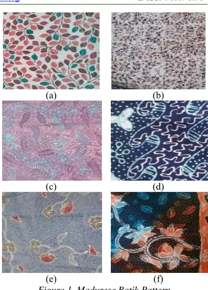
The examples of Madurese batik pattern are shown in Figure 1. In Figure 1, there are six batik patterns. There are plant objects in these patterns. In Figure 1a, leaf object is adopted and combined with curvy stem. In Figure 1b, stem and leaf objects are shown clearly and the pattern is more regular. In Figure 1c, leaf pattern is very dominant with stem and flower objects become its suplements. In Figure 1d, there are stems and leaves with flowers are separated from the tree. In Figure 1e, stem, leaf, and flower are painted unseparately as a tree. In this pattern, plant morphology is very clear. In Figure 1f, stems and flowers are painted together while the leaves are painted separately as background.
Based on examples in Figure 1, it is shown that Madurese batik pattern is dominated by plant objects, especially: stem, leaf, and sometimes flower. Rather than fully stochastics, the plant pattern tends to be deterministic with some stochastic touch. Based on this condition, in this work, we focus on developing Madurese batik pattern model based on curvy plant objects. We also use deterministic approach. Deterministic approach is adopted to match with stamped based batik pattern concept. In stamped based batik, pattern is repeated periodically.
(a) (b)
(c) (d)
(e) (f)
Figure 1. Madurese Batik Pattern
3. COMPUTATIONAL BATIK
Besides using manual process, batik pattern can also be generated by using computational process. Many researches have exploited computational method to generate batik pattern. By using computational method, batik pattern can be generated and modified faster rather than using manual process.
One most popular computational method that is used in generating batik pattern is fractal method. Fractal method is a mathematical model. Basic characteristics of fractal method are self similarity and repetition [15]. By these characteristics, single objects can be replicated. Replication can also be modified in size or orientation so that fractal method is very powerful to make batik pattern from only single object. Besides self similarity, other characteristics of the fractal geometry are self affinity, self inverse, and self squaring [14,15].
[image:3.612.311.524.81.378.2]3560 from a single triangle. Although L-system can be used in replication process, this method is not always used in the fractal model. For example, Marom used Lyapunov function in iteration process to replicate fractal object [15].
In the other side, L-system has been used in some researches in generating batik computationally. Kusuma has used L-system and combined this method with random walk method to make batik pattern that adopts fibrous root pattern [10]. In this work, there are several seeds that fibrous root will grow from them. The growing process of each seed is autonomous relative to other seeds growth. Kusuma has also used L-system in the branching mechanism in generating batik pattern that adopts Acropora morphology [11]. It is because the Acropora growth is similar to common tree where an Acropora contains many branches and some branches can grow from older branch [11].
As it is mentioned in the introduction section, most of researches in computational batik pattern did not refer to any traditional batik pattern. Yulianto, et. al [13], Yulianto, et. al [14], Marom [16], and Hariadi [17] focused on the development of fractal model and combined it with other models in developing batik pattern. All of them did not specify any traditional batik patterns as reference. It means that the replicated objects can be replaced by any traditional batik objects. Meanwhile, Kusuma also focused on the natural objects [10-12] that are adopted and transformed into batik pattern and once again without specifying any traditional batik patterns as reference. One research that exploits traditional batik pattern was held by Wulandari, et. al [17]. They referred La Bako pattern which is the traditional batik pattern from Jember [17]. The special characteristic of La Bako is the adoption of tobacco leaf [17]. Based on this condition, works in developing computational batik that refer to specific traditional batik pattern are potential.
4. PROPOSED MODEL
In this work, we propose four models. Plant parts that we use in this work are: stem, leaf, and flower. These models are developed by using sine wave model as their basis.
Generally, time based sine wave consists of three parts: amplitude (A), frequency (f), and time (t). Amplitude is used to determine the maximum size or magnitude of the wave. Frequency is used to determine how fast a wave
repeates. General sine wave formalization is shown in Equation 1 or Equation 2. In Equation 1, frequency is presented in Hertz. In Equation 2, frequency is converted into wavelength (ω). In both Equation 1 and Equation 2, wave phase is assumed zero. When phase is zero, the value of y at t equals to 0 is 0. So, phase is introduced to make the value of y at t equals to 0 is not 0. The formalization of sine wave with phase (ϕ) is shown in Equation 3. Based on these basic equations, then our proposed models are developed.
t
A
ft
y
sin
2
(1)
t
A
t
y
sin
(2)
t
A
ft
y
sin
2
(3)The first model is simple sinusoid model. The concept of this model is there is array of sine waves that propagates in the same direction. Variation among wave can be the amplitude, wavelength, and or phase. This model can be used for developing background model. In this model, sine wave is generated from the starting point to specific end point. There are four options in this model. First, wave propagates horizontally. Second, wave propagates vertically. Third, wave propagates diagonally. Fourth, wave propagates diagonally with dynamic gradient.
When the sine wave propagates horizontally, the starting point is at x equals to 0. The wave propagates until it reaches the canvas width. After a complete propagated wave is created then the process repeats to create other propagated waves. These propagated waves are arranged vertically. This method is formalized in Equation 4 to Equation 8.
(
s)
sin(
w(
)
(
s))
w
t
y
t
A
x
t
t
y
(4)
t
y
t
y
y
s
s
1
(5)x
t
x
t
x
w(
)
w(
)
(6))
,
(
)
(
min
max
t
s
rand
(7)3561 shown that the phase is determined stochastically and and it ranges between the minimum phase and the maximum phase. The main algorithm for the horizontal propagated wave is shown in Figure 2.
[image:5.612.311.521.228.411.2]The explanation of this algorithm is as follows. Variable px represents the horizontal position of the wave. Variable py represents vertical position of the wave. Variable width represents the canvas width while variable height represents the canvas height. Variable x represents the current horizontal position of the wave while variable y represents the current vertical position of the wave. Variable p represents the phase. In this algorithm, phase is determined stochastically from pmin to pmax and it follows uniform distribution. Variable dx represents the horizontal step size while variable dy represents the vertical step size. The result image of this algorithm is shown in Figure 4a.
begin
py ← 0
while py < height do begin
px ← 0
p ← rand(pmin,pmax)
while px < width do begin
x ← px
y ← py + A * sin(w*x + p)
draw(x,y)
px ← px + dx
end
py ← py + dy
end end
Figure 2. Horizontal Propagated Wave Algorithm
The second option is that the wave propagates vertically. If the wave propagates vertically then the waves are arranged horizontally. Rather than just the phase, in this option, more variables can be set stochastically. This option is formalized by using Equation 8 to Equation 13.
))
(
)
(
sin(
)
(
)
(
)
(
s s w sw
t
x
t
A
t
d
t
t
x
(8))
(
)
1
(
)
(
t
sx
t
sx
t
sx
(9))
,
(
)
(
t
rand
A
minA
maxA
s
(10))
(
).
(
)
(
t
t
y
t
d
w
s w (11)y
t
y
t
y
w(
)
w(
1
)
(12))
,
(
)
(
t
rand
x
minx
maxx
s
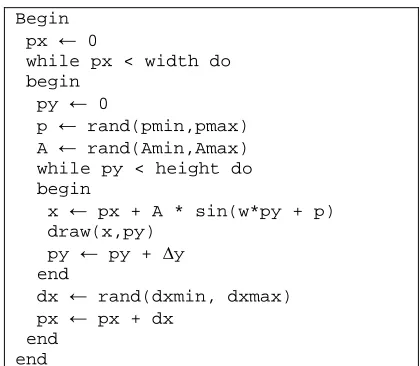
(13)Based on the second option formalization, it is shown that the second option is more stochastic rather than the first option. Besides the phase as it is shown in Equation 7, now the amplitude and the distance between two consecutive waves are also stochastic. Their value ranges from the minimum and the maximum value and it follows uniform distribution. The vertical propagated wave algorithm is shown in Figure 3. Meanwhile, the result image of the vertical propagated wave based pattern is shown in Figure 4b.
Begin
px ← 0
while px < width do begin
py ← 0
p ← rand(pmin,pmax)
A ← rand(Amin,Amax)
while py < height do begin
x ← px + A * sin(w*py + p)
draw(x,py)
py ← py + ∆y
end
dx ← rand(dxmin, dxmax)
px ← px + dx
end end
Figure 3. Vertical Propagated Wave Algorithm
(a) (b)
[image:5.612.88.299.335.504.2](c) (d)
Figure 4. Propagated Wave Based Pattern Result
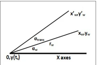
[image:5.612.315.519.444.636.2]3562 angular transformation of point (xw,yw) is related to point (0,y). Point (xw,yw) is transformed as far as the transformation angle (αtrans). So, point (x’w,y’w) now becomes the new wave point.
Figure 5. Angular Transformation Illustration
The transformation process is as follows. First, rw as the distance between point (xw,yw) and point (0,y) is calculated by using Equation 14 to Equation 16. Second, αw as angle of point (xw,yw) related to x axes and point (0,y) is calculated by using Equation 17. The third process is transforming αw to new angle α’w by adding the wave angle with transformation angle. This process if formalized by using Equation 18. Fourth, once the new wave angle is obtained, then the new point (x’w,y’w) is calculated by using Equation 19 and Equation 20. The image result of diagonal wave based pattern that is obtained from angular transformed horizontal propagated wave based pattern is shown in Figure 4c.
2 , 2
,w yw
x
w
d
d
r
(14)w w
x
x
d
,
(15)y
y
d
y,w
w
(16))
arctan(
, ,
w x
w y w
d
d
(17)trans w
w
'
(18)
w ww
r
y
'
.
sin
'
(19))
'
cos(
.
'
wr
w wx
(20)The fourth option is sine wave that propagates diagonally with dynamic gradient. This option is the improvement of the third option. In the third option, transformation angle is set statically. In the fourth option, transformation angle is set dynamic and it follows time based sinusoid pattern.
This transformation angle determination is formalized by using Equation 21.
)
.
sin(
.
)
(
t
transmax transt
trans
(21)In Equation 21, it is shown that the transformation angle is a function of time. The amplitude is the maximum transformation angle. ωtrans is wavelength of the transformation angle. The result is shown in Figure 4d.
[image:6.612.94.295.149.284.2]The second model is lane follower model. In this model, the sine wave propagates by following the lane. Meanwhile, the lane can be straight line or curve. Because the lane can be not a straight line, the wave polarization or the oscilation orientation at time t is perpendicular to the direction of the gradient of the axe at time t. The illustration is shown in Figure 6.
Figure 6. Lane Follower Illustration
In the beginning, lane direction must be calculated. The lane direction is determined by calculating the lane angle (αL). The lane angle is determined by the calculating the gradient of the lane. This concept is diferent to the fourth option in the first model where the transformation angle is relative to point (0,y). This process is formalized in Equation 22 to Equation 26. In Equation 24, mL(t) is the gradient of lane at time t. Equation 26 is used to adjust the angle because tangential value is repeated every 180 degree. Meanwhile, in Equation 27, αtransL(t) is the lane based transformation angle at time t.
)
1
(
)
(
)
(
y
Lt
y
Lt
y
Lt
(22))
1
(
)
(
)
(
x
Lt
x
Lt
x
Lt
(23))
(
)
(
)
(
t
x
t
y
t
m
L L L
3563
))
(
arctan(
)
(
t
m
Lt
L
(25)
else
t
t
x
t
t
L
L L
L
),
(
0
)
(
,
180
)
(
)
(
(26)
(
)
90
)
(
t
Lt
transL
(27)After the lane based transformation angle is determined, the next step is determining the wave position relative to the canvas (xw,yw). Calculating the wave position relative to the canvas cannot be separated from the lane position at time t (xL(t),yL(t)). The magnitude of the wave can be assumed as the nearest distance between the wave and the lane (rw). The wave position is determined by using Equation 28 and Equation 29.
(
)
cos
).
(
)
(
)
(
t
x
t
r
t
t
x
w
L
w
transL (28)
(
)
sin
).
(
)
(
)
(
t
y
t
r
t
t
y
w
L
w
transL (29)Because the wave follows the lane and not any axes, so the time is represented by the lane distance at time t. The lane distance at time t is determined by using Equation 30 to Equation 32. At the beginning, the lane distance equals to 0.
)
(
)
1
(
)
(
t
r
t
r
t
r
L
L
L (30)2
2
(
)
)
(
)
(
t
x
t
y
t
r
L
L
L
(31)0
)
0
(
Lr
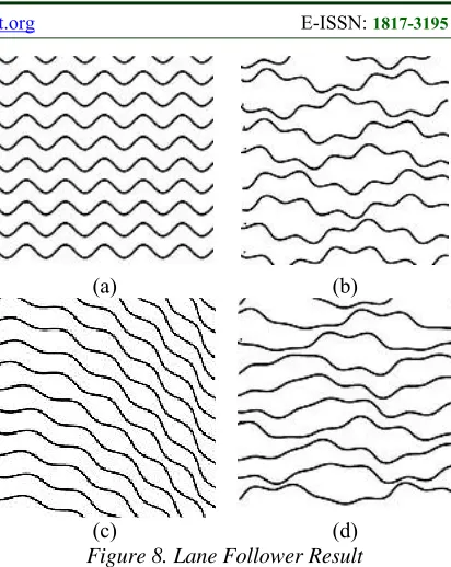
(32)The algorithm of the lane follower model is shown in Figure 7. In Figure 7, the sine wave is assumed as simple sine wave and the angles are presented in degree. The result is shown in Figure 8.
Begin
dyl ← ycur – yprev
dxl ← xcur – xprev
ml ← dyl / dxl
al ← atan(ml)
if dxl < 0 then
al ← al + 180
atransl ← al + 90
dl ← sqrt(pow(dxl,2) + pow(dyl,2))
rl ← rl + dl
rw ← Aw * sin(w*rl + p)
xw ← xcur + rw * cos(atransl)
yw ← ycur + rw * sin(atransl)
[image:7.612.315.521.68.327.2]end
Figure 7. Lane Follower Algorithm
(a) (b)
(c) (d)
Figure 8. Lane Follower Result
[image:7.612.319.523.523.638.2]The third model is the leaf model. In this work, the leaf model is developed as the improvization of the lane follower model. In this third model, the lane is one π radian wave that propagates from zero radian to one π radian. Then, there is a wave that propagates through this lane that the length is π, 3π, 5π, … radian. Because the leaf has two sides, there are two sinusoid lanes that opposite to each other. The illustration is shown in Figure 9. In Figure 9, it is shown that there are two lanes that opposite to each other relative to the leaf direction. The leaf direction is the direction of the leaf relative to the horizontal axe. Besides, there is main leaf angle (αML) that is angle between horizontal axe and leaf direction.
Figure 9. Leaf Model Illustration
[image:7.612.91.297.533.690.2]3564 the leaf. So the leaf lanes are calculated by using Equation 28 to Equation 29. In Equation 28, ALL is the amplitude, ωLL is the wavelength, and tLL is the time of the leaf lane. So, the ωLL.tLL ranges from 0 to π radian. Equation 29 shows that the second lane opposites the first lane.
)
.
sin(
)
(
1 LL LL LL LL
LL
t
A
t
r
(28))
(
)
(
12 LL LL LL
LL
t
r
t
r
(29)After the leaf lanes are created, the next process is transforming the leaf lane position relative to the the main leaf angle. The leaf lane transformation is the rotation as far as main leaf angle with the lane starting point (xSML,ySML) becomes the pivot axis. The transformation process is calculated by using Equation 30 to Equation 39.
ML LL LL LL LLr
t
t
x
1(
)
(
.
).
(30))
(
)
(
11 LL LL LL
LL
t
r
t
y
(31)2 1 2
1
(
)
(
)
)
(
LL LL LL LL LLcurLL
t
x
t
y
t
r
(32))
)
(
)
(
arcsin(
)
(
1 1 LL curLL LL LL LL LLt
r
t
y
t
(33)ML LL
LL LL
tr
LL
t
t
1(
)
1(
)
(34)ML LL
LL LL
tr
LL
t
t
2(
)
1(
)
(35)
(
)
cos
)
(
)
(
11tr LL curLL LL LLtr LL
LL
t
r
t
t
x
(36)
(
)
sin
)
(
)
(
11tr LL curLL LL LLtr LL
LL
t
r
t
t
y
(37)
(
)
cos
)
(
)
(
22tr LL curLL LL LL tr LL
LL
t
r
t
t
x
(38)
(
)
sin
)
(
)
(
22tr LL curLL LL LL tr LL
LL
t
r
t
t
y
(39)The explanation of Equation 30 to Equation 39 is as follows. Creating leaf lane is an iterative process due to the increasing of the tLL. In Equation 30, it is shown that the modification of argument inside the sine function becomes the horizontal position of lane point. Meanwhile, in Equation 31, it is shown that the vertical position of the lane is the result of the calculated lane. Then, the distance of the current lane relative to the lane starting point and the angle of the current lane relative to the x axis are calculated by using Equation 32 and Equation 33. Equation 34 and Equation 35 are used to calculate the leaf lanes transformation angle. Finally, the transformed current lanes position is calculated by using Equation 36 to Equation 39.
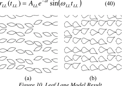
The result is shown in Figure 10. In Figure 10, it is shown that there are two-dimensional array of leaves. There is static value of the vertical and horizontal distance of the leaves relative to their neighbours. In Figure 10, there are two leaf types. The first type is the common leaf as it is shown in Figure 10a. In this type, its lane pattern follows general sine wave. Meanwhile, the second type is leaf model which its lane pattern follows damped sine wave pattern. In general sine wave, the amplitude is static. Meanwhile, in the damped sine wave, the amplitude decrease due to the increasing of the time. The damped sine wave based lane pattern model is formalized by using Equation 40. The damped sine wave based leaf lane model is shown in Figure 10b.
LL LL
at LL LL
LL
t
A
e
t
r
(
)
sin
(40)(a) (b)
Figure 10. Leaf Lane Model Result
After the leaf lane is created, the next step is creating the leaf edge. The leaf edge is modeled by creating the sine wave that propagates through the lane. The leaf edge model is formalized by using Equation 41 to Equation 52. Because the leaf edge direction is perpendicular relative to the lane direction, so the leaf edge direction is the leaf lane direction which is rotated as far as 90 degree as it is shown in Equation 49. In Equation 51 and Equation 52, the current leaf edge position is relative to current lane position.
,...
3
,
2
,
1
,
.
k
t
k
t
L
LL (41),...
3
,
2
,
1
,
.
k
LLk
L
(42))
1
(
)
(
)
(
x
LLt
LLx
LLtrt
LLx
LLtrt
LL (43))
1
(
)
(
)
(
y
LLt
LLy
LLtrt
LLy
LLtrt
LL (44)2
2
(
)
)
(
)
(
L LL LL LL LLL
t
x
t
y
t
r
(45))
)
(
)
(
arctan(
)
(
LL LL LL LL L Lt
x
t
y
t
[image:8.612.316.522.293.438.2]3565
else
t
t
x
t
t
L L
LL LL L
L L
L
),
(
0
)
(
,
)
(
)
(
(47))
sin(
.
)
(
L LW L LLW
t
A
t
r
(48)2
)
(
)
(
Ltrt
L
Lt
L
(49)))
(
cos(
).
(
)
(
L LW L Ltr LL
t
r
t
t
x
(51)))
(
sin(
).
(
)
(
L LW L Ltr LL
t
r
t
t
y
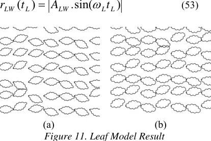
(52)The result is shown in Figure 11. In Figure 11, there are two options of the leaf model. The first option is that the sine wave is the simple wave. Meanwhile the second option is that the sine wave is turned to absolute value. The formalization of the first option is shown in Equation 48 while the formalization of the second option is shown in Equation 53. In Figure 11a, there is not any sharp edge. In the other side, when the leaf model uses Equation 53, there is sharp edge every multiplication of π/2 radian for the argument inside the sine function and the result is shown in Figure 11b.
)
sin(
.
)
(
L LW L LLW
t
A
t
r
(53)(a) (b)
Figure 11. Leaf Model Result
[image:9.612.92.299.394.533.2]The fourth model is the flower model. In this work, the flower is modeled as sine wave that propagates in the circle lane. The flower may contain only one wave or more than one wave. The flower model is illustrated in Figure 12. The flower position is centralized in (xFC, yFC). Then, the flower lane position is determined by the lane distance relative to the flower central (rFL) and the flower lane angle (αF). Then, the flower wave distance is the distance of the wave flower that is relative to the flower central. Meanwhile model formalization is shown in Equation 54 to Equation 58.
Figure 12. Flower Model Illustration
FL F
FL F
FL
(
t
)
(
t
1
)
(54))
(
)
(
)
(
F FL F WFW FFW
t
r
t
r
t
r
(55)))
(
sin(
.
)
(
F FW FW FWFW
t
A
t
r
(56)F F FW F
FW
t
t
(
)
.
(57)))
(
cos(
).
(
)
(
F FW F FW FFW
t
r
t
t
x
(58)))
(
sin(
).
(
)
(
F FW F FW FFW
t
r
t
t
y
(59)The explanation of Equation 54 to Equation 58 is as follows. Equation 54 shows that the behavior of the flower lane angle is incremental by ∆FL. Equation 55 shows that the flower wave distance is the summation of the flower lane distance and the distance of the flower wave relative to the flower lane. In Equation 54 to Equation 56, it is shown that the flower angle step size (∆FW), flower wave amplitude, and the flower lane distance is static. Besides, these variables can be set dynamically. The general algorithm for flower model is shown in Figure 13.
begin set(afl)
while afl < aflmax do begin
rwfw ← Afw * sin(w*t + ph)
rfw ← rfl + rwfw
xfw ← rfw * cos(afl)
yfw ← rfw * sin(afl)
afl ← afl + d_afl
[image:9.612.315.516.542.660.2]end end
Figure 13. Flower Model General Algorithm
3566 rotating process stops when the specified angle distance is reached. The flower model result is shown in Figure 14.
(a) (b)
[image:10.612.89.302.139.353.2](c) (d)
Figure 14. Flower Model Result
In Figure 14, it is shown that there are many variations of the flower although the basic concept is same, which is sine wave. All of flower objects in Figure 14 are arranged in two dimensional arrays. In Figure 14a, a flower is built by using single sine wave with static and same value of lane distance, amplitude, angular speed, and phase. In Figure 14b, a flower is built by using two sine waves which have different amplitude and angular speed. In Figure 14c, flower object is built by using single sine wave with incremental lane distance and dynamic initial phase. In Figure 14d, flower object is built by using single sine wave with sinusoid based dynamic angular speed.
5. IMPLEMENTATION
The proposed model then is implemented into automatic Madurese batik pattern generation application. It is called automatic because user does not need to draw the pattern. User just sets the parameters then the application will generate the Madurese batik pattern based on these set parameters. In this application, a Madurese batik pattern consists of three elements: branch, flower, and flower.
This application is a web based application. It is developed by using PHP language. This application produces image file in jpeg format
[image:10.612.317.521.159.550.2]and this image is also shown in the application. The sample result is shown in Figure 15. This sample pattern is one of much more possible batik patterns that can be generated by using these proposed models.
Figure 15. Madurese Batik Result
3567 There are leaves and flowers between two primary branches. Flowers and leaves appears alternally in stochastic process. The leaf consists of two sine waves that opposite to each other relative to the leaf main lane. Every sine wave that constructs leaf edge propagates as far as 9π radians. The flower is constructed from three sine waves that propagate in rotating lane. The first and the second waves have small amplitude. Meanwhile, the third wave has big amplitude.
6. TESTING
In this section, we will discuss the model performance, especially complexity. The observed variable that is used in the number of executed processes (nexe). In this testing, the canvas size is 2,000 pixels width and 1,000 pixels height.
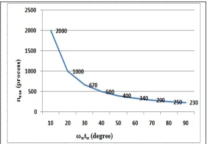
[image:11.612.316.522.300.443.2]The first testing is analyzing complexity in branch creation algorithm. The image is a vertical arranged array of sine waves that propagates horizontally. The vertical distance between consecutive waves is 100 pixels. The adjusted variable is the angular value inside the sinusoid function. The angular value ranges from 10 degree to 90 degree. The step size is 10 degree. The result is shown in Figure 16.
Figure 16. Relation Between Angular Value and Number of Executed Proccesses
In Figure 16, the relation between the angular degree and the number of executed processes is negative potential. When the angular degree is low, the number of executed process is high. Due to the increasing of the angular value, the number of executed process decreases. In the beginning, the decreasing slope is significant so that the number of executed process decreases fast. Then, due to the increasing of the angular degree,
the decreasing slope is low. When the angular degree is high, the reduction of the number of executed process is not significant.
[image:11.612.94.300.443.587.2]The second testing is analyzing the relation between lane length and the algorithm complexity. In this work, lane is important part, because all of sine waves, whether they are stems, leaves, of flowers propagate through the lane. The testing scenario is as follows. The context is leaf creation algorithm. The lane that is observed is the leaf main lane. The leaves can be viewed as two-dimensional array of leaves with static horizontal and vertical distances between consecutive leaves. These distances are 150 pixels. The leaf main lane length ranges from 100 to 200 pixels with the step size is 10 pixels. The result is shown in Figure 17.
Figure 17. Relation Between Lane Length and Number of Executed Proccesses
Figure 17 shows that the relationship between lane length and the number of executed processes is positive linear. It means that the increasing of the lane length is linear to the increasing of the number of executed processes.
7. DISCUSSION
In this section, we will discuss the comparison between this current work and our previous works [10-12] in batik pattern generation. There are four criteria that are used in this section: adoption of traditional batik pattern, smoothness/curviness, direction behavior, and branching behavior. These aspects are important due to several reasons. First, Madurese batik is identical to floral pattern. Second, floral pattern and plant growth are usually smooth and curvy.
3568 crack [12]. In these works, we assumed that these objects are independent to the traditional batik pattern which it means that these objects can be adopted in any traditional batik patterns. In this current work, we change the approach so that we observe and analyze the traditional batik pattern and then we create the computational model so that it can be used to generate new batik pattern that has similar characteristics with the selected traditional pattern.
In the smoothness aspect, this current model performs better than the previous works, especially because these works used random walk method [10,12]. In random walk based model, the direction variation between the current node and the previous node can be various [10]. For example, the previous direction is 30 degree. When the stothastics range is from -20 degree to 20 degree, the current direction can be 10 degree to 50 degree. Suppose that the current direction is 50 degree. So, the next direction can be from 30 degree to 70 degree. Condition in this current work is very different. This model is developed based on sine wave model. Generally, sine wave is continuous so that the appearance is basically smooth too. So, although in this work, this sinusoid is discretized, as long as the step size or sampling period is low, the pattern appearance is still smooth.
In the direction aspect, this sine wave based model is much more predictable rather than the random walk based mode as in previous works [10-12]. Basically, sine wave is deterministic. Besides, the sine wave propagates by following the lane. It means that the propagation direction can be predicted too whether it is linear, quadratic, exponential, or sinusoidal too. This condition is different from random walk model which is basically stochastics although we can add some deterministic aspects. In the plant growth context, it is shown that in the random walk based model, the plant can grow in any directions so that the angle deviation range becomes the growing direction controller.
In branching aspect, this current model is different from the previous models which used Lindenmayer system [10]. In this sinusoid model, the branching model is just an additional feature so that the main branch has one level sub branch. This sub branch is just a single sine wave and cannot trigger another sub branch from it. It is different from the system based model. In previous L-system based plant model, a branch can trigger
another new branch from it based on the probabilistic condition.
Based on the result and comparison between this work and the previous works, major findings in this work are as follows. First, although sine wave is simple and less popular than fractal or L-system, sine wave can also be used to generate floral pattern too, from twig, leaf, and flower. Second, various pattern still can be generated from it by modifying this sine wave become modulated wave. Third, this sine wave is also proven in creating smooth and curvy pattern rather than random walk.
8. CONCLUSION AND FUTURE WORK This work has shown that sine wave based model is better in generating batik pattern smooth and curvy rather than other models in previous works, such as: random walk, graph, and L-system. This work has also shown that although in general, sine wave is deterministic and simple, various patterns still can be generated by modifying this sine wave, for example by using modulated wave. This paper also presents the development of floral pattern by using sine wave based model rather than L-system that is popular and has been adopted in many previous works. These facts show that creating various Madurese batik pattern computationally by using sine wave is possible.
Besides Madurese batik pattern, there are many other traditional batik patterns that can be developed computionally. Some of them are Mega Mendung pattern from Cirebon or Parang pattern from Javanese. So, developing the computational based model of other traditional batik pattern so that these models can be improved, modificated, or manipulated easily can be future research potentials.
REFERENCES:
[1] Y. Rakhmawati, “Batik Madura: Heritage Cyberbranding”, Komunikasi, vol. 9(2), 2015,
pp. 57-65.
[2] J. Sahertian, “Enterpreneurship Perajin Batik Tulis Madura”, Jurnal Entrepreneur dan Entrepeneurship, vol. 5(2), 2016, pp. 45-54.
[3] R.A.S. Suminto, “Batik Madura: Menilik Ciri Khas dan Makna Filosofinya”, Corak Jurnal Seni Kriya, vol. 4(1), 2015, pp. 1-12.
3569
Research International, vol. 9(4), 2018, pp.
12-17.
[5] A. Hindratmo and O.A.W. Riyanto, “Enhancing Capability of Tanjung Bumi Batik Sales Bangkalan Madura”, Kontribusia, vol.
2(1), 2019, pp. 4-8.
[6] A.Y. Putra and Sartini, “Batik Lasem as an Acculturation Symbol of Chinese-Javanese Cultural Values”, Jantra, vol. 11(2), 2016, pp.
115-127.
[7] E. Susilantini, “Digging Up Grandeur Values of Cirebon Batik”, Jantra, vol. 11(2), 2016, pp.
143-153.
[8] Mudjijono, “Lancor Until Mata Keteran (The Motif of Madura Batik)”, Jantra, vol. 11(2),
2016, pp. 169-179.
[9] _, “Batik Nusantara: Batik of the Archipelago”,
Karya Indonesia, 2013, Ministry of Industry of
Indonesia.
[10]P.D. Kusuma, “Fibrous Root Model in Batik Pattern Generation”, Journal of Theoretical and Applied Information Technology, vol. 95(14), 2017, pp. 3260-3269.
[11]P.D. Kusuma, “Simplified Coral Modeling in Batik Pattern Generation”, Journal of Theoretical and Applied Information Technology, vol. 96(10), 2018, pp. 3102-3115.
[12]P.D. Kusuma, “Graph Based Simplified Crack Modeling in Batik Pattern Generation”,
Journal of Theoretical and Applied Information Technology, vol. 95(19), 2017, pp.
5035-5046.
[13]R. Yulianto, M. Hariadi, M.H. Purnomo, and K. Kondo, “Iterative Function System Algorithm Based a Conformal Fractal Transformation for Batik Motive Design”,
Journal of Theoretical and Applied Information Technology, vol. 62(1), 2014, pp.
275-280.
[14]R. Yulianto, M. Hariadi, and M.H. Purnomo, “Fractal Based on Noise for Batik Coloring using Normal Gaussian Method”, IPTEK: The Journal for Technology and Science, vol.
23(1), 2012, pp. 34-40.
[15]S. Marom, “Application of Fractal Concept in Material Batik Development Based on Wolframs Mathematica”, Zero, vol. 1(2), 2017,
pp. 49-61.
[16]Y. Hariadi, M. Lukman, and A.H. Destiarmand, “Batik Fractal: Marriage of Art and Science”, ITB Journal of Visual Art and Design, vol. 4(1), 2013, pp. 84-93.
[17]E.Y. Wulandari, K.D. Purnomo, and A. Kamsyakawuni, “Development of Labako Batik Design with Fractal Geometry Dragon Curve and Tobacco Leaf Motif Combination”,
Jurnal Ilmu Dasar, vol. 18(2), 2017, pp.
125-132.
[18]R.A. Haris, T.W. Purboyo, and P.D. Kusuma, “Several Classification of Batik Art in the World: A Study”, Journal of Engineering and Applied Sciences, vol. 13(21), 2018, pp.
9164-9170.
[19]E. Castellanos, F. Ramos, and M. Ramos, “Semantic Death in Plant’s Simulation Using Lindenmayer Systems”, Proceeding of 10th
International Conference on Natural Computation (ICNC), Xiamen, August 2014,
pp. 360-365.
[20]Suhartono, M. Hariadi, and M.H. Purnomo, “Plant Growth Modeling of Zinnia Elegans Jacq Using Fuzzy Mamdani and L-System Approach with Mathematica”, Journal of Theoretical and Applied Information Technology, vol. 50(1), 2013, pp. 1-6.
[21]D. Leitner and A. Schneff, “Root Growth Simulation Using L-Systems”, Proceeding of Algorithmy, Podbanske, March 2009, pp.
313-320.
[22]A. Davoodi and R.B. Boozarjomehry, “Developmental Model of an Automatic Production of the Human Bronchial Tree Based on L-system”, Computer Methods and Programs in Biomedicine, vol. 132, 2016, pp.
1-10.
[23]P. Prusinkiewicz and A. Lindenmayer, The Algorithmic Beauty of Plants, Springer-Verlag,