ORIGINAL RESEARCH ARTICLE
PREDICTING THE NUMBER OF EMERGENCY ROOM PATIENTS BASED ON AGE GROUP
*
Hannah Ji, Hye Jung Jo and Myung Suk Kim
Sogang Business School, Sogang University
ARTICLE INFO ABSTRACT
Purpose: In this study, we identify the significant variables for each patient group as well as an appropriate model to predict the number of patients by dividing emergency room patients into three age groups (0–14, 15–64, and 65 years or over), where hourly data from an emergency medical care center in Seoul, Korea, are utilized. Methodology/approach: Variables such as day of the week, holiday, weather, and air pollution are used as exogenous variables. The linear model, Poisson regression, auto-regressive with exogenous (ARX) model, and semi-parametric additive-based AR models are used for the prediction analysis. While different variables are identified to be significant according to the patient’s age and prediction model, the variable O3, a compound that can be used to measure air pollution, is significant regardless of the age and model. Findings: We find that the semi-parametric additive-based AR model, which has relatively low mean root mean square error and mean absolute error values compared with other models, is suitable for predicting the number of patients. Finally, the results show that the overall ability to predict the number of patients is higher when categorizing patients by age than considering the total number of patients. Originality: The main contribution is that variable O3 is an important factor and the age group-based semi-parametric forecasting schemes provide an effective result in hourly emergency room patient forecasting.
Copyright © 2018, Hannah Ji et al. This is an open access article distributed under the Creative Commons Attribution License, which permits unrestricted use, distribution, and reproduction in any medium, provided the original work is properly cited.
INTRODUCTION
The number of emergency room (ER) patients is on the rise every year worldwide. Between 2001 and 2011, the number has increased by 2.4% each year on an average. Among the OECD member countries, there has been a high increase rate of ER patients in countries such as Germany, Belgium, the U.K., and New Zealand, while the lowest rate increase in countries such as Chile, Ireland, and the Czech Republic (OECD Health working paper, 2015). In the U.S. in particular, the average number of ER patients has steadily increased from 90.3 million persons in 1993 to 113.9 million in 2003, and around 90% of all ERs in the country have said they have experienced overcrowding during the same 10 years.
*Corresponding author: Hannah Ji, Sogang Business School, Sogang University.
In the case of Korea in 2009, the number of inpatients in emergency medical care centers in Seoul, Korea, exceeded 10 million and it has remained around this number ever since (Emergency Statistics Annual Report, 2013). This large number of inpatients has resulted in overcrowding in the ER, not only causing patient dissatisfaction but also affecting their medical treatment (Schull et al., 2004; Asplin et al., 2006; Bernstein et al., 2009; Cooke et al 2010). To mitigate this issue and utilize the limited resources and labor of medical care centers effectively, it is important to accurately predict the number of patients who visit the ERs (Pines and Hollander,
2008; Asplin et al., 2006). In the case of ERs, it is impossible
to predict the number of patients. That is, you never know how many patients will visit at a specific time. Thus, predicting the number of patients of emergency medical care centers does not only provide useful information to hospitals but also serve as important data for managing hospitals and their staff and providing services. Based on such data, resources and workforce can be efficiently used to help improve general satisfaction of patients and quality of treatment in the ER
(Champion et al., 2007; National Academies Press, 2006). ER
ISSN: 2230-9926
International Journal of Development Research
Vol. 08, Issue, 07, pp.21590-21596, July,2018
Article History: Received 18th April, 2018
Received in revised form 22nd May, 2018
Accepted 17th June, 2018
Published online 30th July, 2018
Available online at http://www.journalijdr.com
Key Words:
Emergency Medical Care Center, Air Pollution,
Hourly Data Forecasting,
Semi-Parametric Additive-Based AR Model
Citation: Hannah Ji, Hye Jung Jo and Myung Suk Kim. 2018. “Predicting the Number of Emergency Room Patients based on Age Group”, International
Journal of Development Research, 8, (07), 21590-21596.
demand prediction studies can be categorized into two types. The first type adopts appropriate prediction models. For
example, Abraham et al. (2009) applied ARIMA and seasonal
ARIMA (SARIMA) models to predict hospitalization services through ER visits and analyze medical resources. However,
while McCarthy et al. (2008) suggested using the Poisson
regression model to predict the number of intraday ER patients
and Jones et al. (2008) argued that the SARIMA model is only
suitable for predicting daily ER patient flows. DíazHierro et al. (2012) further stated that the integrated ARIMA model and harmonic analysis must be used to improve ER care. Kam et al. (2010) argued that the multivariate SARIMA model is the most suitable for predicting daily ER patient flows. The second type of study is based on exogenous variables (e.g., weather and time-series variables) and disease groups that affect the
prediction models of ER patient flows. Lee et al. (2005) stated
that high temperatures affect the number of ER patients,
whereas Jones et al. (2008) showed that among weather
variables, only temperature affects the number of patients. In addition to weather variables, air pollution variables have been used to study respiratory diseases such as asthma, with the study participants mostly being children under 15 years of age (Kim et al., 2010; Walsh et al., 2006). Im et al. (2000) studied the relation between asthma patients and their ER visits using air pollution variables. In addition, Farhat et al. (2005) argued that air pollution variables are related to ER visits as well as hospitalization of children having respiratory problems.
While previous studies have mainly predicted the total number of inpatients, mostly using exogenous variables such as day of the week, holiday, and weather variables, this study is novel from two aspects. First, ER patients are categorized into three age groups (0–14, 15–64, and 65 years or over), termed Groups 1, 2, and 3, respectively, and each group’s significant variables are examined. Choi Byung-chul et al. (2000) have studied the relation between air pollution and respiratory disease patients by dividing the participants into three age groups (a group aged 0–14, another group aged 15–64, and still another group aged 65 or more). Based on that, this study divided its participants into three age groups for analysis. Second, while previous studies have considered only weather variables as exogenous variables when predicting patient number, the importance of environmental pollution is rising. Therefore, it is vital to use air pollution variables not only to study diseases but also to predict and analyze patient number. Therefore, five variables that measure air pollution, namely SO2, NO2, O3, CO, and PM10, are additionally used as
exogenous variables in this study. Further, the auto-regressive with exogenous (ARX) model, Poisson regression model, and semi-parametric addictive-based AR model (a non-linear model) are used to compare and evaluate the predicted number of patients for each group. The remainder of this paper is organized as follows. Section 2 introduces the general characteristics of the data on ER patient number and the variables used in the study. Section 3 describes the model and prediction evaluation method. Section 4 explains the actual data analysis and evaluation of the prediction accuracy of the adopted models. The final section concludes the study.
Data
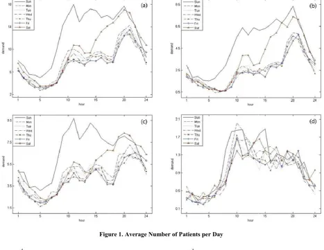
Observations of Data: The participants of this study were the ER patients of a university hospital in Seoul. Time-series data from 12/1/2011 to 1/30/2013 (i.e., 427 days or 10,248 hours) were used for the analysis. Figure 1 demonstrates the pattern
of ER patient flow by hour. Figure 1(a) shows the flow pattern of the total number of patients, illustrating that patient number increases or decreases similarly from Monday to Friday. However, the overall pattern on Saturdays and Sundays is different. The weekday pattern remains until 2 pm on Saturdays, when the number of patients gradually increases over time before decreasing after 8 pm. On Sundays, the number of patients increases again from 7 am, with an average of 15–18 patients checking in from 11 am to 8 pm. Next, we examined the flow pattern of inpatients based on age group. Figure 1(b) shows the inpatient group aged 0–14 years, illustrating that the pattern of these patients from Mondays to Fridays is similar to that of total patients. This number increases on Saturday afternoons, with demand rising substantially on Sundays. As shown in Figure 1(c), the pattern of the 15–64 years group is also similar to that of the entire patient group. While this number increases after 3 pm on Saturdays, it is the highest around 8 pm. In addition, the pattern on Sundays is different from that on the other days, similar to the pattern of Group 1 (aged 0–14 years). Finally, the graph in Figure 1(d), with patients aged 65 or over, demonstrates a contrasting pattern from those in Figures 1(a), 1(b), and 1(c). While the pattern of this group is similar to that of the others on weekdays, this group does not demonstrate such a “weekend effect.” Since the inflow of ER patients differs by age group as well as by the day of the week, this study divided ER patients into three age groups and the effect of the day for each age group was applied as an exogenous variable in the model. Summary statistics for each group by hourly data are reported in Table 1. “Total number” is the number of patients in each group.
Variables
Dependent Variables: In this study, the three age groups (0– 14, 15–64, and 65 years or over) of patients who checked into the ER from 12/1/2011 to 1/30/2013 were the dependent
variables. The dependent variable indicates the number of
patients at k (time) on j (day of the week) (j = 1, 2,…, 7, k = 1,
2,…, 24). Brown et al. (2005) stated that when follows the
Poisson distribution and is converted into = + 0.25,
the distribution approaches normal as increases. Such a
conversion method was used to predict the number of calls at a
call center by Weinberg et al. (2007) and Shin and Kim
(2011). This study also converted , which has the
characteristic of a discrete distribution, into =
+ 0.25, which was then used in the prediction analysis.
This conversion method helped stabilize the distribution.
Further, the converted was applied to the auto-regressive
with exogenous (ARX) and semi-parametric additive-based AR models.
Independent Variables
Time-series variables: This study adopted 24-hour
and weekly seasonal cycles for its time-series variables, which were derived through a spectrum analysis. Further, holiday effect variables were also used as dummy variables.
Weather variables: Weather variables typically
include temperature, humidity, precipitation, and storms, which are regional characteristics. For
instance, Lee et al. (2005) studied the impact of these
study applied the mean values of temperature and humidity in Seoul, as measured by the National Weather Service.
Air pollution variables: Typical air pollution variables
include SO2, NO2, O3, CO, and PM10, which are
measured by the 27 stations of the automatic air quality monitoring network, all located in Seoul. The data are presented as the mean value continuously measured for an hour. This study used the abovementioned air pollution indicators measured from 12/1/2011 to 1/30/2013 at the air quality monitoring station located near the examined emergency medical care center.
Models
Auto Regressive Model: Abraham et al. (2009) applied the ARIMA model to predict hospitalization services through ER visits. Jones (2002) and Zibners et al. (2006) showed that the SARMA model is useful in predicting the total number of ER patients.
The basic AR model is expressed as
1 − ∅ B − ∅ B − ⋯ − ∅ B = .
P was called the order of the AR model and non-negative
integer. The AR model should be no serial correlation and was covariance stationary. This study used the auto-regressive with exogenous (ARX) model, which also has exogenous variables.
Poisson Regression: The Poisson regression model is a generalized linear model that uses independent variables to modify the frequency or count of the dependent variable. The Poisson regression model in this study is described in the
equation below. Here (expected value) indicates the
frequency of the incidents per period, and log functions are used because the Poisson distribution is always greater than 0.
The log of is expressed as the exponential sum of the
independent variables:
log = + + + ⋯ + .
Farhat et al. (2005) stated that patients who visit or check into the ER are considered as count events that follow the Poisson distribution and hence used the Poisson regression model. In addition, Schwarts (2013) assumed that the errors follow the Poisson distribution in the regression analysis.
Semi-Parametric Additive: The semi-parametric additive model is used when the relationship between the independent and dependent variables is non-linear. The following basic formula of the semi-parametric additive model, in which
function is predicted using the smoothing spline method, is
used:
= + ( ) + ( ) + ⋯ + ( ) + .
In this study, the time-series lag and holiday effect were predicted using the parametric method, while the temperature, humidity, and air pollution variables were predicted and analyzed using the smoothing spline method.
For example, the formula for the number of patients in Group 3 (aged 65 or over) is as follows:
Evaluation of the Prediction Ability of the Models
This study used the method described in Weinberg et al.
(2007) as its evaluation standard of prediction accuracy. The two equations below calculate the root mean square error
(RMSE) and mean absolute error (MAE) per j day:
is used in the auto-regressive with exogenous (ARX) model and semi-parametric additive-based AR models to calculate the number of ER patients predicted at k (hour) on j (day) as
= − 0.25. is the predicted value of =
+ 0.25. Here, k is 24 because the study data were
observed for a day (i.e., 24 hours). A prediction was made every hour for 24 hours, and the evaluation was analyzed each day. The prediction period for the number of patients on the following day was 30 days (from 1/1/2013 to 1/30/2013).
Therefore, j = 1, 2,…, 30, and 30 RMSE and MAE values each
were predicted. The prediction accuracy of the models was then evaluated based on this result using the mean of these values. This study used in-sample and out-of-sample testing in the analysis to predict the model and evaluate its prediction ability, respectively. The initial in-sample data were obtained from 12/1/2011 to 12/31/2012 (9,528 hours) and the out-of-sample data were from 1/1/2013 to 1/30/2013 (720 hours). In addition, the in-sample data were updated every day (24 hours). The specific prediction evaluation of a model can be applied in the following steps:
Step 1: Using the initial in-sample data, find the time lag and exogenous variable that affect the model.
Step 2: Using the model formula based on the significant variables found in the in-sample data, predict the number of patients for the next day by hour (24) and calculate the RMSE and MAE of the corresponding day.
Step 3: Update the range of the in-sample data each day (24 examined values) and repeatedly predict the number of patients by hour the following day.
Step 4: Obtain the RMSE and MAE for 30 days in total to evaluate the accuracy of the predicted values for each model.
RESULTS
Estimation
Before conducting the prediction analysis, the augmented Dickey–Fuller unit root test was performed to see whether the time-series data of this study were stationary. The data were identified to be stationary and, thus, appropriate for the time-series analysis. Then, the time-time-series data were analyzed to check for significant cycles. First, Bartlett’s Kolmogorov– Smirnov statistics were used to conduct the white noise test, which showed that the cycles were significant.
Figure 1
Figure 2. Periodogram of the Number of Patients by Group Figure 1. Average Number of Patients per Day
Table 1. Descriptive Statistics of Data
Total Patients Group 1 Group 2 Group 3
mean 8.6259 2.9490 4.7160 0.9609
standard deviation 5.1080 2.6257 2.9297 1.0974
median 8 2 4 1
min 0 0 0 0
max 40 24 24 7
[image:5.595.96.499.196.293.2]total number 88,398 30,221 48,330 9,847
Table 2. Regression Model Prediction Value of the In-Sample Data
Variable Total Patients Group 1 Group 2 Group 3
(Intercept) 8.5274 2.7322 4.7641 1.2368
Holiday 5.3339 2.1870 2.7731 0.3527
Temperature 0.0701 0.0287 0.0348 0.0060
Humidity −0.0527 −0.0235 −0.0211 −0.0092
CO 1.1376 0.7456 0.5451
O3 43.8335 26.8222 13.4524 3.0932
NO2 16.3819 9.5747 3.3495
SO2 −20.8173
[image:5.595.98.497.333.431.2]PM10
Table 3. Poisson Regression Prediction Value of the In-Sample Data
Lag Total Patients Group 1 Group 2 Group 3
(Intercept) 2.1591 1.0474 1.5520 0.2102
Holiday 0.4867 0.5526 0.4742 0.3153
Temperature 0.0079 0.0093 0.0072 0.0066
Humidity −0.0061 −0.0080 −0.0044 −0.0096
CO 0.1252 0.2217 0.0843
O3 4.2082 6.9624 2.5767 2.4761
NO2 1.6838 2.4471 0.8131 2.9011
SO2 −7.4023 6.7688
PM10 0.0005
Table 4. AR model with Exogenous Prediction Value of the In-Sample Data
Lag Total Patients Group 1 Group 2 Group 3
(Intercept) 1.4629 0.6430 1.2407 0.5779
24 0.0331 0.0527 0.0351 0.0438
48 0.0178 0.0263 0.0226 0.0437
96 0.0175 0.0303 0.0207 0.0342
168 0.0623 0.0917 0.0570 0.0449
Holiday 0.6537 0.4645 0.4801 0.1178
Temperature 0.0021 0.0024 0.0021 0.0017
Humidity −0.0025 −0.0028 −0.0018 −0.0026
CO 0.0705 0.0840
O3 2.9356 2.9021 1.9873 0.9839
NO2 0.8517
SO2
PM10
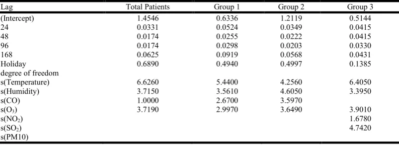
Table 5. Semi-parametric Additive-based AR Model Prediction Value of the In-Sample Data
Lag Total Patients Group 1 Group 2 Group 3
(Intercept) 1.4546 0.6336 1.2119 0.5144
24 0.0331 0.0524 0.0349 0.0415
48 0.0174 0.0255 0.0222 0.0415
96 0.0174 0.0298 0.0203 0.0330
168 0.0625 0.0919 0.0568 0.0431
Holiday 0.6890 0.4940 0.4997 0.1385
degree of freedom
s(Temperature) 6.6260 5.4400 4.2560 6.4050
s(Humidity) 3.7150 3.5610 4.6050 3.3950
s(CO) 1.0000 2.6700 3.5970
s(O3) 3.7190 2.9970 3.6490 3.9010
s(NO2) 1.6780
s(SO2) 4.7420
s(PM10)
[image:5.595.100.497.472.608.2] [image:5.595.98.500.642.788.2]The spectrum analysis was then conducted to find more specific cycles, and the statistics showed a significant result. Figure 2(a) is the periodogram used to find the seasonal cycle of the total number of patients. The figure shows that the most significant cycle (period), which is the largest periodogram, was 24 and the second most significant period was 168. This finding indicates that the data of this study with the spectrum analysis have a consistent variability for 24 and 168. Figures 2(b), 2(c), and 2(d) demonstrate the periodograms by age. The significant period of patients in Group 1 (aged 0–14 years) was the same as that of the total number of patients. The most significant periods of Group 2 (aged 15–64) and Group 3 (aged 65 or over) were also 24, and the second most significant periods were 12 for both.
In the temporal data, the number of daily (weekly) intervals was 24 (168), indicating that the total number of patients has daily and weekly intervals. Therefore, the number of ER patients has seasonal characteristics by day and week. The prediction analysis was conducted using the daily and weekly intervals found in the periodogram. When selecting specific variables, only the time-series model lags applied to the initial in-sample data and significant exogenous variables below a significance level of 0.05 were selected. Tables 2–5 summarize the variables that affect the number of patients. Holiday, a time-series variable, weather variables, and ozone (O3), an air
pollution variable, were found to be significant for all groups of the four models. In addition, Group 3 (aged 65 or over)
showed that O3 and NO2 had an impact regardless of the model
type. Different variables influenced the number of patients, depending on the prediction model.
Prediction: Tables 6 and 7 summarize the prediction evaluation result for each model, showing that accuracy increased as the mean values of the RMSE and MAE decreased. The result of the prediction model also showed that the mean values of the RMSE and MAE of the semi-parametric additive-based AR model were the lowest of the four models. This finding indicated thatnon-linear exogenous variables that affect the number of patients must be considered.
Conclusion
This study aimed to find the most suitable model for predicting the inflow of emergency medical care center patients by age.
For the analysis, the hourly number of inpatients, which was the dependent variable, was divided by age while exogenous variables such as time-series variables, weather variables, and air pollution variables were used as independent variables. Then, the predicted patient numbers were compared and evaluated using three models with significant variables. As a result, holiday, a time-series variable, weather variables, and ozone (O3), an air pollution variable, were confirmed to have
an impact regardless of the prediction model and age. This result shows that O3 has an important role in predicting the
number of patients. In addition, while NO2 was significant in
Group 3 (aged 65 or over). Therefore, ER patients aged 65 or over become affected not only by O3 but also by NO2. The
goodness-of-fit result of the prediction model was as follows. All groups, including total patients, showed that the mean values of the RMSE and MAE of the semi-parametric additive-based AR model were the smallest. This finding indicated that it would be more convenient to use non-linear exogenous variables than linear variables. In addition, selecting the appropriate model for each age group of patients would increase the accuracy when predicting the number of emergency medical care center patients.
REFERENCES
Abraham, G., Byrnes, G., Bain, C.A. 2009. Short-term
Forecasting of Emergency Inpatient Flow, IEEE
Transactions on Information Technology in Biomedicine
13(3), 380-388
Asplin, B.R., Flottemesch, T.J., Gordon, B.D. 2006. Developing Models for Patient Flow and Daily Surge
Capacity Research, Academic Emergency Medicine 3(11),
1109-1113
Bernstein, S.L., Aronsky, D., Duseja, R., et al. 2009. The Effect of Emergency Department Crowding on Clinically Oriented Outcomes, Society for Academic Emergency Medicine 16(1), 1-10
Byung-chul Choi, Jung Wan Koo, Sung Kyun Park, et al.
2000. Time Series Analysis between the Concentration of Air Pollutants and the Number of Respiratory Disease
Outpatients in Seoul, Korean Journal of Occupational and
Environmental Medicine 12(1), 70-80
[image:6.595.82.509.79.155.2]Cooke David, Rohleder Thomas, Rogers Paul 2010. A dynamic model of the systemic causes for patient treatment
Table 6. Mean Values of the RMSE for the Predicted Number of Patients
RMSE Total Patients Number of Patients by Group (by age)
Total Aged 0–14 Aged 15–64 Aged 65 over
(88,398) (30,221) (48,330) (9,847)
Linear regression 4.3772 2.0833 2.8404 1.1131
Poisson 7.6901 2.5238 4.5526 1.4963
Auto regression 3.5694 1.8292 2.5884 1.1205
[image:6.595.82.508.196.266.2]Semi-parametric 3.5438 1.8120 2.5688 1.1211
Table 7. Mean Values of the MAE for the Predicted Number of Patients
MAE Total Patients Number of Patients by Group (by age)
Total Aged 0–14 Aged 15–64 Aged 65 over
(88,398) (30,221) (48,330) (9,847)
Linear regression 3.4014 1.6097 2.2125 0.8167
Poisson 6.2458 1.7167 3.6514 1.0000
Auto regression 2.6792 1.2708 1.9583 0.7750
delays in emergency departments, Journal of Modelling in Management 5(3), 287-301
Díaz-Hierro, J., Martín Martín, J.J., Vilches Arenas, A, et al. 2012. Evaluation of Time-seriesModels for Forecasting
Demand for Emergency Health Care Services,
Emergencies 24(3), 181-188
Farhat, S.C., Paulo, R.L., Shimoda, T.M., Conceição, G.M. et
al. 2005. Effect of Air Pollution on Pediatric Respiratory Emergency Room Visits and Hospital Admissions,
Brazilian Journal of Medical and Biological Research
38(2), 227-235
Hye Jin Kam, Jin Ok Sung, Rae Woong Park 2010. Prediction of Daily Patient Numbers for a Regional Emergency Medical Center using Time Series Analysis, Healthcare Informatics Research 16(3), 158-165
Jang Young Lee, Jin Hong Min, Jung Soo Lee, et al. 2005. The Impact of Day and Weather Characteristics on the Number of ER Patients, Korea Emergency Medical Journal 16(2), 287-291
Jones SS., Thomas A., Evans RS., Welch SJ., Haug PJ., Snow GL. 2008. Forecasting Daily Patient Volumes in the Emergency Department, Academic Emergency Medicine 15(2),159-170
McCarthy, M.L., Zeger, S.L., Ding, R., Aronsky, D., Hoot, N.R., Kelen, G.D. 2008. The Challenge of Predicting
Demand for Emergency Department Services, Academic
Emergency Medicine 15(4), 337-346
Myung Suk Kim 2011. A Comparison of Seasonal Linear Models and Seasonal ARIMA Models for Forecasting Intra -day Call Arrivals, Communications of the Korean Statistical Society 18(2), 237-244
Pines, J.M., Hollander, J.E. 2008. Emergency Department Crowding Is Associated with PoorCare for Patients with
Severe Pain, Annals of Emergency Medicine 51(1), 1-5
Sang Hun Kim, Ji Young Sohn, Jong Tae Lee, et al. 2010. The
Impact of Air Pollution in Seoul on Adult Asthma: Cross-patient Study, Korea Internal Medicine Bulletin 78(4) Schull MJ, Vermeulen M, Slaughter G, Morrison L, Daly P
2004. Emergency Department Crowding and Thrombolysis Delays in Acute Myocardial Infarction, Annals of Emergency Medicine 44(6), 577-585
Taek Su Shin, Myung Suk Kim 2011. Predicting the Amount of Intra-Day Calls at the Call Center Using Spectrum Analysis and Seasonal Linear Model, Korea Statistics Society24(2), 217-225
Taylor, J.W. 2008. A Comparison of Univariate Time Series Methods for Forecasting Intraday Arrivals at a Call Center, Management Science 54(2), 253-265
Walsh, T.L., Frezieres, R.G. 2006. Patterns of Emergency Contraception Use by Age and Ethnicity from a Randomized Trial Comparing Advance Provision and Information Only, Contraception 74(2), 110-117
Weinberg, J., Brown D., Stroud R. 2007. Bayesian Forecasting of an Inhomogeneous Poisson Process with Applications to
Call Center Data, Journal of the American Statistical
Association 102(480), 1185-1198