Novel Image Watermarking Algorithm with DWT SVD

(1)

Novel Image Watermarking Algorithm with DWT-SVD

N.Anil Kumar

PG Student QISCET, Ongole,

A.P., India.

M.Haribabu

Asst.professor QISCET, Ongole,

A.P., India.

Ch.Hima Bindu

Professor, QISCET, Ongole, A.P., India.

ABSTRACT

This paper presents a novel watermarking scheme based on Discrete Wavelet Transforms and Singular Value Decomposition. The singular values of HL band is going to embedded with watermark singular values making use of scaling factor (α).The effectiveness of the proposed algorithm is measured using peak signal to noise ratio (PSNR), structural similarity index(SSIM) and normalized correlation (NC) factors. The robustness of the proposed algorithm is tested by performing various attacks like Salt & Pepper noise, Gaussian noise and rotation etc on watermarked image. The experimental results show both the robustness and high fidelity of the algorithm.

Keywords

Discrete Wavelet Transform, Singular Value Decomposition, Quality metrics.

1. INTRODUCTION

The rapid growth of technology needs the ownership protection of multimedia data. Hence, the technology of image watermarking has recently attracted increasing interests [1, 2, 3]. This embeds the watermark image into the host data to attain the objective of protection. For extracting watermark can be classified into two different groups: blind detection and non-blind detection watermarking. The blind detection means to extract watermark without the help of the original host image and the original watermark. On the contrary, the non-blind detection requires the original host image or the original watermark [4-7].

For embedding more information and better robustness against the common attacks can be achieved through transform-domain approach. Earlier embedding watermark in spatial domain has the advantages of low computational complexity and easy implementation. However, this is generally fragile to common image processing operations or other attacks. In order to overcome these shortcomings, the method based on singular value decomposition (SVD) has been becoming one of the research hot fields. The SVD-based watermarking method has three advantages as follows: (1) the size of the matrix from SVD transformation is not fixed; (2) when a small perturbation is added to an image, larger variation of its singular values does not occur; (3) singular values represent intrinsic algebraic image properties [8,9,22]. By considering these advantages there are various techniques developed based on SVD with another transform domain [13, 14, 18]. For example [14, 18] follows the above process with a hybrid DWT–SVD domain watermarking scheme

considering human visual system properties. They decompose the host image into four sub-bands and apply SVD to each sub-band and embed singular values of the watermark into these sub-bands [10].

2. IMAGE TRANSFORMS

2.1 Discrete Wavelet Transform (DWT)

DWT provides a framework in which an image is decomposed, with each level corresponding to lower frequency sub band, and higher frequency sub bands. There are two main groups of transforms: continuous and discrete. In one dimension the idea of the wavelet transform is to present the signal as a superposition of wavelets. If a signal is represented by f(t), the wavelet decomposition is

)

(

)

(

, ,

,

t

f

n

m mn

n m

c







(1)

Where

t

m



m

t

n



n

m





 

2

,

(

)



, m and n are

integers. There exist very special choices of  such that

) (

,nt m



constitutes an ortho normal basis, so that the wavelet transform coefficient can be obtained by an inner calculation:



  

 f t f t dt

n m n

m n

m

c

, () ()

, ,

,



(2)

In order to develop a multiresolution analysis, a scaling function



is needed, together with the dilated and

translated parameters of



t n



t m m

n

m  

 

2

, ( )



. The signal f(t) can

be decomposed in its coarse part and details of various sizes by projecting it onto the corresponding spaces. Therefore, the

approximation coefficients

a

m,n_{of the function} f _at

resolution

2

m

and wavelet coefficients

c

m,n

can be

obtained:

a

h

a

m k

k

k n n

m,





2  1, (3)

a

g

_m _k

k n k

n m

C

, 1 2

, 



_ _ (4)

Where

h

n_{is a low pass FIR filter and}

g

n is a high pass

FIR filter. To reconstruct the original signal, the analysis filter can be selected from a biorthogonal set which have a related set of synthesis filters. These synthesis filters h~_andg~_can

(2)



_   _    

n n l mn n l mn

l

m f

h

a

f

g

c

f

a

( ) ( ) _, ( )

2 ,

1

~

(5)

[image:2.595.73.283.142.256.2]

Equations (3) and (4) are implemented by filtering and down sampling. Conversely (5) is implemented by an initial up sampling and a subsequent filtering [21].

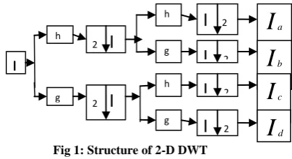
Fig 1: Structure of 2-D DWT

In a 2-D DWT, a 1-D DWT is first performed on the rows and then columns of the data by separately filtering and down sampling. This result in one set of approximation coefficients

a

I _{and three set of detail coefficients, as shown in Figure 1,} where

I

b_,

I

c_,

I

d_{represent the horizontal, vertical and}

diagonal directions of the image , respectively. In the filter theory, these four sub images correspond to the outputs of low-low (LL), low-high (LH), high-low (HL), and high-high (HH) bands. By recursively applying the same scheme to the LL sub band multi resolution decomposition with a desire level can then be achieved. There, a DWT with K. Decomposition levels will have M=3*K+1 such frequency bands. Above figure (see Figure 1) shows the 2-D structures of the wavelet transform with two decomposition levels. It should be noted that for a transform with K levels of decomposition, there is always only one low frequency band, the rest of bands are high frequency bands in a given decomposition level [11].

2.2 Singular Value Decomposition

The SVD for square matrices was discovered independently by Beltrami in 1873 and Jordan in 1874, and extended to rectangular matrices by Eckart and Young in the 1930s. It was not used as a computational tool until the 1960s because of the need for sophisticated numerical techniques. In later years, Gene Golub demonstrated its usefulness and feasibility as a tool in a variety of applications [16].

A be an image matrix of size N×N. Using SVD the matrix A can be decomposed as:





r i T i i i T A A

A

S

V

u

s

v

U

A

1

(6)

UA= [u1, u2,u3…..uN] (7) VA= [v1, v2,v3…..vN] (8)















N A

S

..

0

0 .

.

0 ..

...

0

0 .

....

0

2 1 (9)

Where r is the rank of matrix A, UA and VA are orthogonal matrices of size N×N, whose column vectors are ui and vi. S is an N×N diagonal matrix containing the singular values si assumed to be in decreasing order. S1 ≥S2≥ ………. ≥S r > 0 and r = rank (A). S1, S2 . . . , Sr are the square roots of the Eigen values of ATA. They are called the singular values of A [12, 13, 14 ]. SVD is one of the most useful tools of linear algebra with several applications in image compression, and other signal processing fields[22].

The result of SVD gives good accuracy, good robustness and good imperceptibility in resolving the rightful ownership of watermarked image [15].

3. PROPOSED METHOD

The Proposed method is explained with embedding and extraction process. For this consider the host image(A) with 256 ˟ 256 size and watermark image(b) with 128 ˟ 128 size. First start with embedding and later continue with extraction process

3.1 Watermark Embedding Process

The watermark embedding algorithm is as follows:

1) Apply the discrete wavelet transform (DWT), on cover image A to decompose into four sub bands LL, HL, LH, and HH.

A= (LL, LH, HL, HH) (10) 2) Apply SVD on HL sub band

[ui si vi]=svd (HL) (11)

3) Apply SVD on binary watermark image (b)

[ub sb vb]=svd(b) (12)

4) Now perform the embedding process on above singular values (sb and si) to provide embedded singular component (s1).















else

j

i

sb

j

i

si

j

i

sb

j

i

si

j

i

sb

j

i

si

j

i

s

)

,

(

*

)

,

(

)

,

(

)

,

(

)

,

(

*

)

,

(

)

,

(

1 



(13)

5) Pertain inverse SVD on above s1

aw= ui*s1*vi'; (14) 6) Apply the inverse DWT using modified HL coefficient

(aw) and remaining coefficients (LL, LH, HH) to produce the watermarked image (IW).

I

h

g

2

I

2

I

h

g

h

g

I

2

I

2

I

2

I

2

I

a

I

b

I

c

(3)

[image:3.595.54.289.67.307.2]

Fig 2: Proposed embedding flowchart

3.2 Watermarking Extraction process

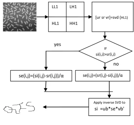
The watermark is extracted by considering the watermarked image (IW), singular values of host image and scaling parameter α. The process of extraction is given below: 1) Apply DWT to decompose the watermarked (and

possibly with and without attacks) cover image (IW) into four sub bands LL1, HL1, LH1, and HH1. IW= LL1, LH1, HL1, HH1 (15) 2) Apply SVD to HL1 sub band image.

[ur sr vr]=svd (HL1) (16)

3) The watermark extraction process is given below by considering all input parameters















else

j

i

si

j

i

sr

j

i

sr

j

i

si

j

i

sr

j

i

si

j

i

se



/

))

,

(

)

,

(

)

,

(

)

,

(

/

))

,

(

)

,

(

)

,

(

(17)

4) Apply inverse SVD to the se to get the extracted watermark image (b1).

[image:3.595.317.548.69.283.2]

b1=ub*se*vb'; (18)

Fig 3: Proposed extracting flowchart

4. EXPERIMENTAL RESULTS

The experimental simulation is carried out using MATLAB 7.1. Various standard images are considered to study the effects of perceptibility and robustness of the watermarking algorithm. The standard test images are grayscale images and a binary watermark image is having size 128x128. The embedding process is applied on above images and the resultant image is called watermarked image. To show the robustness of the proposed algorithm various attacks (Gaussian, salt & pepper, rotation etc..) are applied on watermarked image. The resultant and input images are shown below(see Figure 4&5). The performance of the proposed algorithm is evaluated by using Peak Signal to Noise Ratio (PSNR), Normalized Correlation (NC) and Structural Similarity Index (SSIM). The difference between cover image and watermarked image is used to estimate the watermark imperceptibility. The above values are tabulated (see Table-1, 2, 3) for various images. The respective plots of images are also shown below (see Figure 6-8).

4.1 Peak signal to Noise Ratio (PSNR)

PSNR (Peak Signal to Noise Ratio) is a metric for the ratio between the maximum possible power of a signal and power of corrupting noise that affects the fidelity of its representation. It is used to measure the quality of reconstructed images.

]

))

,

(

)

,

(

1 )

255 (

[

*

10 )

(

₁

0 1

0 2

10

log





 







_M

m N

n

m

F

n

m

R

MN

db

PSNR

(19)

The PSNR is computed between input image and watermarked image after applying various attacks.

LL1 LH1

HL1 HH1

[ur sr vr]=svd (HL1)

Apply inverse SVD to

si =ub*se*vb'

IF si(i,j)>sr(i,j)

se(i,j)=(si(i,j)-sr(i,j))/α se(i,j)=(sr(i,j)-si(i,j))/α

yes

no

LL LH

HL HH

HH

[ui si vi]=svd (HL)

Apply inverse SVD to s1

aw=ui*s1*vi';

Apply IDWT to LL,LH,aw and HH [ub sb vb]=svd (b) IF _{si(i,j)>sb(i,j)}

s1(i,j)=si(i,j)-αsb(i,j) s1(i,j)=si(i,j)+αsb(i,j)

(4)

4.2 Normalized correlation (NC)



   



_M

i N

j M

i N

j

i

WI

j

i

EWI

j

i

WI

NC

1 1

2

1 1

)

]

,

[

(

])

,

[

]

,

[

(

(20)

Where WI [i, j] is the original watermark image and EWI [i, j] is the extracted watermark image .M is the height and N is the width of the image. The NC is computed between the watermark and extracted watermark image after attacks. The NC shows the robustness of the algorithm. Its value is 1.0000 before the watermark image is attacked.

The results for different attacks are shown(see table 2). In order to investigate the robustness watermarked image was attacked by various attacks.

4.3 The SSIM Algorithm

The Structural Similarity Index was first proposed in [19]. The application of algorithm is that it matches human subjectivity. In particular, both the SSIM Index and the HVS are highly sensitive to degradations in the spatial structure of image luminance. The basic SSIM algorithm compared between two images which to be properly aligned and scaled point by point.

The computations are performed by sliding a NxN (typically 11x11) Gaussian weighted window. SSIM is more accurate and consistence than MSE and PSNR despite the cost more. This algorithm computes three similarity functions on the windowed image data are: luminance similarity, contrast similarity, and structural similarity.

The three similarity functions are then combined into the general form of the SSIM index [20]:

SSIM(x; y) = [l(x; y)]α . [c(x; y)]β. [s(x; y)]r (21) The SSIM is computed between the input image and watermarked image after applying various attacks.

Fig 4: (a) Original Image, (b) Watermark Image, (c) Watermarked Image

Fig 5: (a) Salt &Pepper noise 0.005 (b) Salt &Pepper noise 0.01 (c) Gaussian noise 0.001 (d) Gaussian noise 0.002 (e)

Rotation noise 300 (f) Rotation noise 450

(a)

(b)

(c)

(d)

(e)

_(f)

(a)

(b)

[image:4.595.333.526.78.295.2] [image:4.595.313.581.346.551.2]

(5)

[image:5.595.314.566.73.228.2]

Table 1: PSNR for Various Images FOR Different Attacks

Table 2: NC for Various Images for Different Attacks

Table 3: SSIM for Various Images for Different Attacks

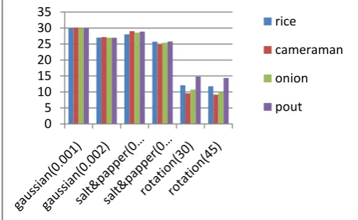
Fig 6: Plot of Various Images PSNR Value

Fig 7: Plot of Various Images NC Value

Fig 8: Plot of Various Images SSIM Value

0 5 10 15 20 25 30 35

rice

cameraman

onion

pout

0 0.1 0.2 0.3 0.4 0.5 0.6 0.7 0.8 0.91

rice

cameraman

onion

pout

0 0.1 0.2 0.3 0.4 0.5 0.6 0.7 0.8

0.91 rice

cameraman

onion

pout

Type of Image

Gaussia n Noise (0.001)

Gaussia n Noise (0.002)

Salt & pepper Noise (0.005)

Rotation (300)

Rotation (450)

Rice. 29.99 27.02 28.01 25.70 12.07 11.75

Camer

aman 30.11 27.18 29.00 24.80 9.61 9.15

Onion 29.96 26.98 28.57 25.39 10.76 10.03

Pout 30.01 26.96 28.85 25.79 14.80 14.35

Type of Image

Gaussi an Noise (0.001)

Gaussia n Noise (0.002)

Rotation (300₎

Rotation (450₎

Rice. 0.8282 0.7286 0.8967 0.8407 0.1375 0.1234

Camer

aman 0.7120 0.5969 0.8995 0.7719 0.3109 0.2744

Onion 0.6483 0.5010 0.8636 0.7460 0.3602 0.3375

Pout 0.6119 0.4514 0.8386 0.7082 0.5131 0.5040 Type

of Image

Gaussia n Noise (0.001)

Gaussia n Noise (0.002)

Rotatio

n(300₎ Rotatio_n(450₎

Rice. 0.7097 0.7145 0.7320 0.7306 0.6120 0.9148

Camer

aman 0.3954 0.4548 0.4592 0.5270 0.3252 0.7246

Onion 0.6689 0.7196 0.7733 0.7779 0.8346 0.6718

(6)

5. CONCLUSION

The proposed watermarking algorithm is non blind watermarking scheme. The extraction process requires singular values of the host image and scaling factor to extract watermark. By using this proposed method the PSNR, NC, SSIM are 88.24, 1.0000, and 1.0000 respectively before the attacks. It is concluded that the embedding and extraction of the proposed method is robust, high fidelity and shows improvement over the existed method. This method can be extended with multi scale Discrete Wavelet Transforms or setting of automatic scaling factor or applying multiple times of Singular Value Decomposition etc to achieve effective watermarking scheme.

The effectiveness of the watermarking algorithm can be achieved by changing various embedding process. The effectiveness of the watermarking process can be increased by using various embedding techniques. In addition to this the robustness of the algorithm can be evaluated for the same.

6. REFERENCES

[1] H. Luo, F. Yu, Z.L. Huang, Z.M. Lu, “Blind image watermarking based on discrete fractional random transform and sub sampling”, Optik 122 (2011), 311– 316.

[2] D.C. Lou, H.K. Tso, J.L. Liu, “A copyright protection scheme for digital images using visual cryptography technique”, Comput. Stand. Interfaces 29 (2007)125– 131.

[3] Qingtang Su, Yugang Niu, Qingjun Wang, Guorui Sheng, “A blind color image watermarking based on DC component in the spatial domain”, Optik 124(2013), 6255-6260.

[4] C.C. Lai, A digital watermarking scheme based on singular value decomposition and tiny genetic algorithm, Digit Signal Process. 21 (2011) 522–527. [5] X.Y. Luo, D.S. Wang, P. Wang, F.L. Liu, “A review

on blind detection for image Steganography”, Signal Process. 88 (2008) 2138–2157.

[6] T.K. Tsui, X.P. Zhang, D. Androutsos, Color image watermarking using multidimensional Fourier transforms, IEEE Trans. Inform. Forensics Secur. 3 (2008) 16–28.

[7] Qingtang Su, Yugang Niu, Xianxi Liu, Tao Yao, “A novel blind digital watermarking algorithm for embedding color image into color image” Optik 124(2013), 3254-3259.

[8] R. Liu, T. Tan, An SVD-based watermarking scheme for protecting rightful ownership, IEEE Trans. Multimed. 4 (2002) 121–128.

[9] Shao-li Ji, “A novel blind color images watermarking based on SVD”, Optik 125 (2014) 2868-2874.

[10]Yong Yang, Dong Sun Park, and Shuying Huang. “Medical Image Fusion via an Effective Wavelet Based Approach”.

[11]A. Ranade, S.S. Mahabalarao, S. Kale, A variation on SVD based image compression, Image Vision Comput. 25 (6) (2007) 771–777.

[12]R.Z. Liu, T.N. Tan, An SVD-based watermarking scheme for protecting rightful ownership, IEEE Trans. Multimedia 4 (1) (2002) 121–128.

[13]M. Narwaria, W. Lin, SVD-based quality metric for image and video using machine learning, IEEE Trans. Syst. Man Cybern. B Cybern. 42 (2) (2012) 347– 364. [14]seema,sheetal sharma, “DWT-SVD based efficient

image watermarking algorithm to achieve high robustness and perceptual quality”, ijarcsse, vol 2, issue 4, april 2012.

[15]Deepa Mathew k “svd based image watermarking scheme”,ijcaecot 2010.

[16] D. Kahaner, C. Moler and S. Nash, Numerical Methods and Software (New Jersey: Prentice-Hall, Inc, 1989).

[17]U. M. Gokhale, Y. V. Joshi” A New Watermarking Algorithm Based on Image Scrambling and SVD in the Wavelet Domain” ACEEE Int. J. on Network Security , Vol. 02, No. 03, July 2011 © 2011 ACEEE DOI: 01.IJNS.02.03.141

[18] Navnidhi Chaturvedi Dr S.J. Basha “A Novel SVD based Digital Watermarking Scheme using DWT and A comparative study with DWT-Arnold, SVD-DCT and SVD-DFT based watermarking”, ijdacr Volume 1, Issue 4, November 2012.

[19] Z. Wang, A. C. Bovik, H. R. Sheikh, and E. P. Simoncelli, “Image quality assessment: From error visibility to structural similarity,” IEEE Trans. Image Processing,vol. 13, pp. 600–612, Apr 2004.

[20] Zhou Wang,Alan C.Bovik and Hamid R.Sheikh “ “Structural similarity Based Range Image Quality Assessment”, Digital Video image quality and perceptual coding, Nov 2005.

[21] Neha K. Kothadiya , Udesang K. Jaliya , Vikram M. Agrawal “Image Fusion Based on Consistency Checking and Salience Match Measure”, (IJETT) - Volume4Issue4- April 2013.