Research Article An Impulse Dynamic Model for Computer Worms

(1)

Volume 2013, Article ID 286209,8pages http://dx.doi.org/10.1155/2013/286209

Research Article

An Impulse Dynamic Model for Computer Worms

Chunming Zhang, Yun Zhao, and Yingjiang Wu

School of Information Engineering, Guangdong Medical College, Dongguan 523808, China Correspondence should be addressed to Chunming Zhang; [email protected] Received 3 May 2013; Accepted 2 June 2013

Academic Editor: Luca Guerrini

Copyright © 2013 Chunming Zhang et al. This is an open access article distributed under the Creative Commons Attribution License, which permits unrestricted use, distribution, and reproduction in any medium, provided the original work is properly cited.

A worm spread model concerning impulsive control strategy is proposed and analyzed. We prove that there exists a globally

attractive virus-free periodic solution when the vaccination rate is larger than𝜃₁. Moreover, we show that the system is uniformly

persistent if the vaccination rate is less than𝜃₁. Some numerical simulations are also given to illustrate our main results.

1. Introduction

Computer virus is a kind of computer program that can replicate itself and spread from one computer to others including viruses, worms, and trojan horses. Worms use system vulnerability to search and attack computers. As hardware and software technologies develop and computer networks become an essential tool for daily life, worms start to be a major threat. In June 2010, the Belarusian security firm Virus Block Ada discovered deadly Stuxnet worm. The Stuxnet worm is the first known example of a cyber-weapon that is designed not just to steal and manipulate data but to attack a processing system and cause physical damage. The Stuxnet worm is the first cyber-attack of its kind and has infected thousands of computer systems worldwide.

Consequently, the trial on better understanding the worm propagation dynamics is an important matter for improving the safety and reliability in computer systems and networks. Similar to the biological viruses, there are two ways to study this problem: microscopic and macroscopic. Following a macroscopic approach, since [1,2] took the first step towards modeling the spread behavior of worms, much effort has been done in the area of developing a mathematical model for the worms propagation [3–13]. These models provide a reasonable qualitative understanding of the conditions under which viruses spread much faster than others and why.

In [7], the authors investigated a differentialSEIRmodel by making the following assumptions (Figure 1).

A population size𝑁(𝑡), that is, the total nodes at any time

𝑡in the computer network, is partitioned into subclasses of

nodes which are susceptible, exposed (infected but not yet infectious), infectious, and recovered with sizes denoted by

𝑆(𝑡),𝐸(𝑡),𝐼(𝑡), and𝑅(𝑡), respectively. One has 𝑁 (𝑡) = 𝑆 (𝑡) + 𝐸 (𝑡) + 𝐼 (𝑡) + 𝑅 (𝑡) , 𝑆󸀠(𝑡) = 𝑏 − 𝜆𝐼𝑆 − 𝑝𝑏𝐸 − 𝑞𝑏𝐼 − 𝑑𝑆 + 𝜁𝑅, 𝐸󸀠(𝑡) = 𝜆𝐼𝑆 + 𝑝𝑏𝐸 + 𝑞𝑏𝐼 − 𝜀𝐸 − 𝑑𝐸, 𝐼󸀠(𝑡) = 𝜀𝐸 − 𝛾𝐼 − 𝑑𝐼 − 𝜂𝐼, 𝑅󸀠(𝑡) = 𝛾𝐼 − 𝜁𝑅 − 𝑑𝑅, (1)

where 𝑏, 𝑑, and 𝜆 are positive constants and𝜀, 𝜂, 𝛾, 𝜁are nonnegative constants. The constant𝑏is the recruitment rate of susceptible nodes to the computer network,𝑑is the per capita natural mortality rate (i.e., the crashing of nodes due to the reason other than the attack of worms),𝜀is the rate constant for nodes leaving the exposed class𝐸for infective class𝐼,𝛾is the rate constant for nodes leaving the infective class𝐼for recovered class𝑅,𝜂is the disease related death rate (i.e., crashing of nodes due to the attack of worms) in the class

𝐼, and𝜁is the rate constant for nodes becoming susceptible again after recovering.

In theSEIRSmodel, the flow is from class𝑆to class𝐸, class 𝐸 to class𝐼, class 𝐼 to class 𝑅, and again class 𝑅 to class 𝑆. For the vertical transformation, we assume that a fraction𝑝and a fraction𝑞of the new nodes from the exposed and the infectious classes, respectively, are introduced into

(2)

S 𝜆IS I 𝛾I R 𝜁R dS dI dR b 𝜀E pbE E dE qbI +

Figure 1: Original model.

the exposed class 𝐸. Consequently, the birth flux into the exposed class is given by𝑝𝑏𝐸 + 𝑞𝑏𝐼, and the birth flux into the susceptible class is given by𝑏 − 𝑝𝑏𝐸 − 𝑞𝑏𝐼.

As we know, antivirus software is a kind of computer program which can detect and eliminate known worm. There are two common methods to detect worms: using a list of worm signature definition and using a heuristic algorithm to find worm based on common behaviors. It has been observed that it does not always work in detecting a novel worm by using the heuristic algorithm. On the other hand, obviously, it is impossible for antivirus software to find a new worm signature definition on the dated list. So, to keep the antivirus software in high efficiency, it is important to ensure that it is updated. Based on the previous facts, we propose an impulsive system to model the process of periodic installing or updating antivirus software on susceptible computers at fixed time for controlling the spread of worm.

Based on the previous facts, we propose the following assumptions:

(H1) the antivirus software is installed or updated at time

𝑡 = 𝑘𝜏 (𝑘 ∈ 𝑁), where𝜏is the period of the impulsive effect;

(H2)𝑆computers are successfully vaccinated from𝑆class to𝑅class with rate𝜃 (0 < 𝜃 < 1).

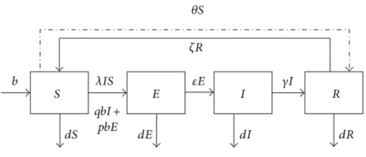
According to the previous assumptions (H1)-(H2) and for the reason of simplicity, we propose the following model (Figure 2): 𝑆󸀠(𝑡) = 𝑏 − 𝜆𝐼𝑆 − 𝑝𝑏𝐸 − 𝑞𝑏𝐼 − 𝑑𝑆 + 𝜁𝑅, 𝐸󸀠_{(𝑡) = 𝜆𝐼𝑆 + 𝑝𝑏𝐸 + 𝑞𝑏𝐼 − 𝜀𝐸 − 𝑑𝐸,} 𝐼󸀠_{(𝑡) = 𝜀𝐸 − 𝛾𝐼 − 𝑑𝐼 − 𝜂𝐼,} 𝑅󸀠(𝑡) = 𝛾𝐼 − 𝜁𝑅 − 𝑑𝑅, 𝑡 ̸= 𝑘𝜏, 𝑘 ∈ 𝑍+, 𝑆 (𝑡+_{) = (1 − 𝜃) 𝑆 (𝑡) ,} 𝐸 (𝑡+_{) = 𝐸 (𝑡) ,} 𝐼 (𝑡+_{) = 𝐼 (𝑡) ,} 𝑅 (𝑡+_{) = 𝑅 (𝑡) + 𝜃𝑆 (𝑡) ,} 𝑡 = 𝑘𝜏, 𝑘 ∈ 𝑍+. (2) The total population size𝑁(𝑡)can be determined by𝑁(𝑡) =

𝑆(𝑡) + 𝐸(𝑡) + 𝐼(𝑡) + 𝑅(𝑡)to form the differential equation

𝑁󸀠_{(𝑡) = 𝑏 − 𝑑𝑁 (𝑡) − 𝜂𝐼 (𝑡) ,} ₍₃₎ S 𝜆IS I 𝛾I R 𝜁R dS dI dR b 𝜀E pbE E dE 𝜃S qbI +

Figure 2: Impulse model.

which is derived by adding the equations in system (1). Thus the total population size𝑁may vary in time. From (2), we have

𝑏 − (𝑑 + 𝜂) 𝑁 (𝑡) ≤ 𝑁󸀠(𝑡) ≤ 𝑏 − 𝑑𝑁 (𝑡) . (4) It follows that

𝑏

(𝑑 + 𝜂) ≤𝑥 → ∞lim inf𝑁 (𝑡) ≤𝑥 → ∞lim sup𝑁 (𝑡) ≤

𝑏 𝑑.

(5) The system (2) can be reduced to the equivalent system

𝑆󸀠_{(𝑡) = 𝑏 − 𝜆𝐼𝑆 − 𝑝𝑏𝐸 − 𝑞𝑏𝐼 − 𝑑𝑆} + 𝜁 (𝑁 − 𝑆 − 𝐸 − 𝐼) , 𝐸󸀠_{(𝑡) = 𝜆𝐼𝑆 + 𝑝𝑏𝐸 + 𝑞𝑏𝐼} − 𝜀𝐸 − 𝑑𝐸, 𝐼󸀠_{(𝑡) = 𝜀𝐸 − 𝛾𝐼 − 𝑑𝐼 − 𝜂𝐼,} 𝑁󸀠_{(𝑡) = 𝑏 − 𝑑𝑁 (𝑡) − 𝜂𝐼 (𝑡) ,} 𝑡 ̸= 𝑘𝜏, 𝑘 ∈ 𝑍+_, 𝑆 (𝑡+_{) = (1 − 𝜃) 𝑆 (𝑡) ,} 𝐸 (𝑡+_{) = 𝐸 (𝑡) ,} 𝐼 (𝑡+) = 𝐼 (𝑡) , 𝑁 (𝑡+) = 𝑁 (𝑡) . 𝑡 = 𝑘𝜏, 𝑘 ∈ 𝑍+, (6) The initial conditions for (6) are

𝑆 (0+) > 0, 𝐸 (0+) > 0, 𝐼 (0+) > 0, 𝑁 (0+) > 0.

(7) From physical considerations, we discuss system (6) in the closed set Ω = {(𝑆, 𝐸, 𝐼, 𝑁) ∈ 𝑅₊4 | 0 ≤ 𝑆 + 𝐸 + 𝐼 ≤ 𝑏 𝑑, 0 ≤ 𝑁 ≤ 𝑏 𝑑} . (8) The organization of this paper is as follows. InSection 2, we establish sufficient condition for the local and global attractivity of virus-free periodic solution. The sufficient condition for the permanence of the model is obtained in Section 3. Some numerical simulations are performed in Section 4. In the final section, a brief conclusion is given, and some future research directions are also pointed out.

(3)

2. Global Attractivity of Virus-Free

Periodic Solution

To prove our main results, we state three lemmas which will be essential to our proofs.

Lemma 1 (see [14]). Consider the following impulsive

differen-tial equations:

̇𝑢 (𝑡) = 𝑎 − 𝑏𝑢 (𝑡) , 𝑡 ̸= 𝑘𝜏,

𝑢 (𝑡+) = (1 − 𝜃) 𝑢 (𝑡) , 𝑡 = 𝑘𝜏, (9)

where𝑎 > 0,𝑏 > 0, and0 < 𝜃 < 1. Then system(9)has a unique positive periodic solution

𝑢_𝑒(𝑡) = 𝑎

𝑏+ ( 𝑢∗− 𝑎

𝑏) 𝑒−𝑏(𝑡−𝑘𝜏), 𝑘𝜏 < 𝑡 ≤ (𝑘 + 1) 𝜏,

(10)

which is globally asymptotically stable; there𝑢∗= 𝑎(1 − 𝜃)(1 −

𝑒−𝑏𝜏)/𝑏(1 − (1 − 𝜃)𝑒−𝑏𝜏).

If𝐼(𝑡) ≡ 0, we have the following limit systems:

𝑆󸀠_{(𝑡) = 𝑏 − 𝜆𝐼𝑆 − 𝑝𝑏𝐸 − 𝑞𝑏𝐼} − 𝑑𝑆 + 𝜁 (𝑁 − 𝑆 − 𝐸) , 𝐸󸀠(𝑡) = 𝑝𝑏𝐸 − 𝜀𝐸 − 𝑑𝐸, 𝑁󸀠_{(𝑡) = 𝑏 − 𝑑𝑁,} 𝑡 ̸= 𝑘𝜏, 𝑘 ∈ 𝑍+_, 𝑆 (𝑡+_{) = (1 − 𝜃) 𝑆 (𝑡) ,} 𝐸 (𝑡+_{) = 𝐸 (𝑡) ,} 𝑁 (𝑡+) = 𝑁 (𝑡) . 𝑡 = 𝑘𝜏, 𝑘 ∈ 𝑍+_, (11)

When𝑝𝑏−𝑑−𝜀 < 0, there exists𝑡₁when𝑡 > 𝑡₁, lim_{𝑡 → ∞}𝐸(𝑡) =

0. From the third and sixth equations of system (11), we have lim_{𝑡 → ∞}𝑁(𝑡) = 𝑏/𝑑. We have the following limit systems:

𝑑𝑆 𝑑𝑡 = (1 − 𝑝) 𝑏 + V𝑏 𝜇 − (𝜇 +V) 𝑆, 𝑡 ̸= 𝑘𝑇, 𝑘 ∈ 𝑍+, 𝑆 (𝑡+) = (1 − 𝜃) 𝑆 (𝑡) , 𝑡 = 𝑘𝑇. (12)

According toLemma 1, we know that periodic solution of system (12) is of the form

𝑆_𝑒(𝑡) = (𝜇 (1 − 𝑝) +_{𝜇 (𝜇 +}_V₎V) 𝑏

+ (𝑆∗−(𝜇 (1 − 𝑝) +V) 𝑏

𝜇 (𝜇 +V) ) 𝑒−(𝜇+V)(𝑡−𝑘𝜏), 𝑘𝜏 < 𝑡 ≤ (𝑘 + 1) 𝜏,

(13)

and it is globally asymptotically stable, where𝑆∗ = ((1−𝑝)𝑏+

(V𝑏/𝜇))(1 − 𝜃)(𝑒(𝜇+V)𝜏− 1)/(𝜇 +V)(𝑒(𝜇+V)𝜏− 1 + 𝜃).

Theorem 2. Let (𝑆(𝑡), 𝐸(𝑡), 𝐼(𝑡), 𝑁(𝑡)) be any solution of

system(6)with initial values𝑆(0+) > 0,𝐸(0+) > 0,𝐼(0+) > 0,

and𝑁(0+) > 0; then(𝑆_𝑒(𝑡), 0, 0, 𝑏/𝑑)is locally asymptotically stable, provided that𝑝𝑏 − 𝑑 − 𝜀 < 0and𝑅₀< 1, where

𝑅₀= 1 (𝑑 + 𝜀 − 𝑝𝑏) (𝛾 + 𝑑 + 𝜂) 𝜏 − 𝜀𝑞𝑏𝜏 × 𝜀𝜆_𝑑𝑏[𝜏 + 𝜃 (1 − 𝑒 (𝜁+𝑑)𝜏₎ (𝜁 + 𝑑) (𝑒(𝜁+𝑑)𝜏_{− 1 + 𝜃)}] . (14)

Proof. The local stability of virus-free periodic solution may be determined by considering the behaviors of a small amplitude perturbation of the solution. Define𝑤(𝑡) = 𝑆(𝑡) −

𝑆_𝑒(𝑡),𝑥(𝑡) = 𝐸(𝑡),𝑦(𝑡) = 𝐼(𝑡), and𝑧(𝑡) = 𝑁(𝑡)−𝑏/𝑑, and then the linearized system of system (6) reads as

𝑤󸀠_{(𝑡) = − (𝑑 + 𝜁) 𝑤 (𝑡) − (𝑝𝑏 + 𝜁) 𝑥 (𝑡)} − (𝜆𝑆_𝑒(𝑡) + 𝜁 + 𝑞𝑏) 𝑦 (𝑡) + 𝜁𝑧 (𝑡) , 𝑥󸀠(𝑡) = (𝑝𝑏 − 𝑑 − 𝜀) 𝑥 (𝑡) + (𝑞𝑏 + 𝜆𝑆𝑒(𝑡)) 𝑦 (𝑡) , 𝑦󸀠_{(𝑡) = 𝜀𝑥 (𝑡) − (𝑟 + 𝑑 + 𝜂) 𝑦 (𝑡) ,} 𝑧󸀠_{(𝑡) = −𝜂𝑦 (𝑡) − 𝑑𝑧 (𝑡) ,} 𝑡 ̸= 𝑘𝜏, 𝑘∈𝑍+_, 𝑤 (𝑡+) = 𝑤 (𝑡) , 𝑥 (𝑡+) = 𝑥 (𝑡) , 𝑦 (𝑡+) = 𝑦 (𝑡) , 𝑧 (𝑡+_{) = 𝑧 (𝑡) .} 𝑡 = 𝑘𝜏, 𝑘 ∈ 𝑍+_, (15) LetΦ(𝑡)be the fundamental solution matrix of system (15), and thenΦ(𝑡)must satisfy

𝑑Φ (𝑡) 𝑑𝑡 = ( −𝑑 − 𝜁 −𝑝𝑏 − 𝜁 −𝜆𝑆_𝑒(𝑡) − 𝜁 − 𝑞𝑏 𝜁 0 𝑝𝑏 − 𝑑 − 𝜀 𝑞𝑏 + 𝜆𝑆_𝑒(𝑡) 0 0 𝜀 −𝑟 − 𝑑 − 𝜂 0 0 0 −𝜂 −𝑑 ) Φ (𝑡) ̇= 𝐴Φ (𝑡) , (16) and Φ(0) = 𝐼, the identity matrix. We can easily see that two eigenvalues of the matrix𝐴are−𝑑 − 𝜁and−𝑑, and the other two eigenvalues are determined by the 2×2 matrix𝐵 =

(𝑝𝑏−𝑑−𝜀 𝑞𝑏+𝜆𝑆𝑒(𝑡)

𝜀 −𝑟−𝑑−𝜂 ). Denote the eigenvalues of𝐵as𝜆1,𝜆2, and then as𝑝𝑏−𝑑−𝜀 < 0, we have𝜆₁+𝜆₂= 𝑝𝑏−𝑑−𝜀−𝑟−𝑑−𝜂 < 0,

𝜆₁𝜆₂= (𝑝𝑏 − 𝑑 − 𝜀) (−𝑟 − 𝑑 − 𝜂) − 𝜀 (𝑞𝑏 + 𝜆𝑆_𝑒(𝑡)) .

(4)

Therefore, by the Floquet theorem [15], (𝑆_𝑒(𝑡), 0, 0, 𝑏/𝑑) is locally asymptotically stable, provided that

𝐺 = ∫𝜏 0 [(𝑝𝑏 − 𝑑 − 𝜀) (−𝛾 − 𝑑 − 𝜂) − 𝜀 (𝑞𝑏 + 𝜆𝑆𝑒(𝑡))] 𝑑𝑡 = (𝑝𝑏 − 𝑑 − 𝜀) (−𝛾 − 𝑑 − 𝜂) 𝜏 − 𝜀𝑞𝑏𝜏 − 𝜀𝜆𝑏_𝑑[𝜏 + 𝜃 (1 − 𝑒 (𝜁+𝑑)𝜏₎ (𝜁 + 𝑑) (𝑒(𝜁+𝑑)𝜏_{− 1 + 𝜃)}] > 0. (18) When𝑅₀= (1/((𝑑+𝜀−𝑝𝑏)(𝛾+𝑑+𝜂)𝜏−𝜀𝑞𝑏𝜏))𝜀𝜆(𝑏/𝑑)[𝜏+𝜃(1−

𝑒(𝜁+𝑑)𝜏_{)/(𝜁 + 𝑑)(𝑒}(𝜁+𝑑)𝜏_{− 1 + 𝜃)] ≤ 1}_{, the previous inequality} is satisfied for𝑝𝑏 − 𝑑 − 𝜀 < 0.

The proof is complete.

Theorem 3. If𝑅₁≤ 1, and𝑝𝑏−𝑑−𝜀 < 0then(𝑆_𝑒(𝑡), 0, 0, 𝑏/𝑑)

is globally asymptotically stable for system(11), where

𝑅₁= 1 (𝑑 + 𝜀 − 𝑝𝑏) (𝛾 + 𝑑 + 𝜂) 𝜏 − 𝜀𝑞𝑏𝜏𝜀𝜆 𝑏𝜏 𝑑 × [1 − 𝜃 (𝑒(𝜁+𝑑)𝜏_{− 1 + 𝜃)}] . (19)

Proof. Because𝑒𝑥− 1 > 𝑥, for𝑥 > 0, we have

𝑅₀< 𝑅₁. (20)

ByTheorem 2, we know that(𝑆_𝑒(𝑡), 0, 0, 𝑏/𝑑)is locally asymp-totically stable. In the following, we will prove the global attraction of(𝑆_𝑒(𝑡), 0, 0, 𝑏/𝑑). Let 𝐿 = 𝜀𝐸 − (𝑝𝑏 − 𝜀 − 𝑑) 𝐼. (21) Then 𝐿󸀠= 𝜀𝐸󸀠− (𝑝𝑏 − 𝜀 − 𝑑) 𝐼󸀠, 𝐿󸀠= [𝜀𝜆𝑆 + 𝜀𝑞𝑏 + (𝑝𝑏 + 𝜀 − 𝑑) (𝑟 + 𝑑 + 𝜂)] 𝐼. (22)

Therefore,(𝑆_𝑒(𝑡), 0, 0, 𝑏/𝑑) is globally asymptotically stable, provided that 𝐿󸀠= ∫𝜏 0 [𝜀𝜆𝑆 + 𝜀𝑞𝑏 + (𝑝𝑏 + 𝜀 − 𝑑) (𝑟 + 𝑑 + 𝜂)] 𝐼 𝑑𝑡 < 0, 𝐿󸀠= ∫𝜏 0 [𝜀𝜆𝑆 + 𝜀𝑞𝑏 + (𝑝𝑏 + 𝜀 − 𝑑) (𝑟 + 𝑑 + 𝜂)] 𝑑𝑡 < [𝜀𝑞𝑏 + (𝑝𝑏 + 𝜀 − 𝑑) (𝑟 + 𝑑 + 𝜂)] 𝜏 + 𝜀𝜆𝑏 𝑑(1 − 𝜃 𝑒(𝑑+𝜁)𝜏_{− 1 + 𝜃}) 𝜏 < 0. (23) When𝑅₁= (1/((𝑑 + 𝜀 − 𝑝𝑏)(𝛾 + 𝑑 + 𝜂)𝜏 − 𝜀𝑞𝑏𝜏))𝜀𝜆(𝑏𝜏/𝑑)[1 −

𝜃/(𝑒(𝜁+𝑑)𝜏− 1 + 𝜃)] ≤ 1, the previous inequality is satisfied. The proof is complete.

Corollary 4. The virus-free periodic solution(Se(t), 0, 0,b/d)

of system(6)is globally attractive, if𝜃 > 𝜃₁, where𝜃₁ = 1 −

𝑒(𝜁+𝑑)𝜏_{+ 𝜀𝑏𝜆(𝑒}(𝜁+𝑑)𝜏_{− 1)/𝑑[(𝑑 + 𝜀 − 𝑝𝑏)(𝑟 + 𝑑 + 𝜂) − 𝜀𝑞𝑏]}_. Theorem 2 determines the global attractivity of (6) in

Ω for the case𝑅₀ < 1. Its realistic implication is that the infected computers vanish, so the worms are removed from the network.Corollary 4implies that the computer virus will disappear if the vaccination rate is less than𝜃₁.

3. Permanence

In this section, we say that the worm is local if the infected population persists above a certain positive level for suffi-ciently large time. The local of worm can be well captured and studied through the notion of permanence.

Definition 5. System (6) is said to be uniformly persistent if there is an𝜑 > 0(independent of the initial data) such that every solution (𝑆(𝑡), 𝐼(𝑡), 𝑅(𝑡), 𝑁(𝑡)) with initial conditions (8) of system (6) satisfies

lim

𝑡 → ∞inf𝑆 (𝑡) ≥ 𝜑, 𝑡 → ∞lim inf𝐼 (𝑡) ≥ 𝜑, lim

𝑡 → ∞inf𝑅 (𝑡) ≥ 𝜑, 𝑡 → ∞lim inf𝑁 (𝑡) ≥ 𝜑.

(24)

Theorem 6. Suppose that𝑅₁ > 1and𝑝𝑏 − 𝑑 − 𝜀 < 0. Then

there is a positive constant𝑚_𝐼such that each positive solution

(𝑆(𝑡), 𝐸(𝑡), 𝐼(𝑡), 𝑅(𝑡))of system(6)satisfies 𝐼(𝑡) ≥ 𝑚_𝐼, for t large enough.

Proof. Now, we will prove that there exist 𝑚_𝐼 > 0 and a sufficiently large𝑡_𝑝such that𝐼(𝑡) ≥ 𝑚_𝐼holds for all𝑡 > 𝑡_𝑝. Suppose that𝐼(𝑡) < 𝐼∗for all𝑡 > 𝑡₀. From the forth equation of (6), we have 𝑏 − 𝑑𝑁 (𝑡) > 𝑁󸀠_{(𝑡) > 𝑏 − 𝑑𝑁 (𝑡) − 𝜂𝐼}∗_, 𝑏 𝑑 > 𝑁 (𝑡) > 𝑏 − 𝜂𝐼∗ 𝑑 . (25)

From the second equation of (6), we have

𝐸󸀠_{(𝑡) = 𝜆𝐼𝑆 + 𝑝𝑏𝐸 + 𝑞𝑏𝐼 − 𝜀𝐸 − 𝑑𝐸} < 𝜆𝐼∗𝑆 + 𝑞𝑏𝐼∗+ (𝑝𝑏 − 𝜀 − 𝑑) 𝐸 < 𝜆𝐼∗𝑏 𝑑 + 𝑞𝑏𝐼∗+ (𝑝𝑏 − 𝜀 − 𝑑) 𝐸. (26) As𝑝𝑏 − 𝑑 − 𝜀 < 0, 𝐸 (𝑡) < _{𝑑 (𝜀 + 𝑑 − 𝑝𝑏)}(𝑞𝑏 + 𝜆) 𝑏𝐼∗ . (27)

(5)

From the first equation of (6), we have 𝑆󸀠(𝑡) = 𝑏 − 𝜆𝐼𝑆 − 𝑝𝑏𝐸 − 𝑞𝑏𝐼 − 𝑑𝑆 + 𝜁 (𝑁 − 𝑆 − 𝐸 − 𝐼) > 𝑏 + 𝜁𝑏 − 𝜂𝐼∗ 𝑑 − 𝑞𝑏𝐼∗− 𝜁𝐼∗ − (𝑝𝑏 + 𝜁) (𝑞𝑏 + 𝜆) 𝑏𝐼∗ 𝑑 (𝜀 + 𝑑 − 𝑝𝑏)− (𝜆𝐼∗+ 𝑑 + 𝜁) 𝑆 (𝑡) . (28) Consider the following comparison system:

V󸀠(𝑡) = 𝑏 + 𝜁𝑏 − 𝜂𝐼_𝑑 ∗ − 𝑞𝑏𝐼∗− 𝜁𝐼∗ − (𝑝𝑏 + 𝜁)_{𝑑 (𝜀 + 𝑑 − 𝑝𝑏)}(𝑞𝑏 + 𝜆) 𝑏𝐼∗ − (𝜆𝐼∗+ 𝑑 + 𝜁)V(𝑡) , 𝑡 ̸= 𝑘𝜏, V(𝑡+) = (1 − 𝜃)V(𝑡) , 𝑡 = 𝑘𝜏, V(0+) = 𝑆 (0+) . (29) let𝐴 ̇= 𝑏+𝜁((𝑏−𝜂𝐼∗)/𝑑)−𝑞𝑏𝐼∗−𝜁𝐼∗−(𝑝𝑏+𝜁)((𝑞𝑏+𝜆)𝑏𝐼∗/𝑑(𝜀+ 𝑑 − 𝑝𝑏)),𝐵 ̇= 𝜆𝐼∗+ 𝑑 + 𝜁.

ByLemma 1, we know that there exists𝑡₁> 𝑡₀such that

V(𝑡) = 𝐴 𝐵 + (V∗− 𝐴 𝐵) 𝑒−𝐵(𝑡−𝑘𝜏), 𝑘𝜏 < 𝑡 ≤ (𝑘 + 1) 𝜏, V∗= 𝐴 (1 − 𝜃) (1 − 𝑒 −𝐵𝜏₎ 𝐵 (1 − (1 − 𝜃) 𝑒−𝐵𝜏₎, 𝑆 (𝑡) >V(𝑡) ̇= 𝑆∗> 0, for𝑡 > 𝑡₁. (30) From the second equation of (6), we have

𝐸󸀠(𝑡) = 𝜆𝐼𝑆 + 𝑝𝑏𝐸 + 𝑞𝑏𝐼 − 𝜀𝐸 − 𝑑𝐸 > 𝜆𝐼∗𝑆∗+ 𝑞𝑏𝐼∗− (𝜀 + 𝑑 − 𝑝𝑏) 𝐸,

𝐸 (𝑡) > 𝜆𝐼_{𝜀 + 𝑑 − 𝑝𝑏}∗𝑆∗+ 𝑞𝑏𝐼∗.

(31)

From the third equation of (6); we have

𝐼󸀠(𝑡) = 𝜀𝐸 − 𝛾𝐼 − 𝑑𝐼 − 𝜂𝐼 > 𝜀𝜆𝐼∗𝑆∗+ 𝑞𝑏𝐼∗

𝜀 + 𝑑 − 𝑝𝑏 − (𝛾 + 𝑑 + 𝜂) 𝐼.

(32)

Note that𝑅₁> 1, we have

𝐼 (𝑡) > _{𝛾 + 𝑑 + 𝜂}𝜀 𝜆𝐼_{𝜀 + 𝑑 − 𝑝𝑏}∗𝑆∗+ 𝑞𝑏𝐼∗ > 𝐼∗. (33) This contradicts𝐼(𝑡) ≤ 𝐼∗. Hence, we can claim that for any

𝑡₀> 0, it is impossible that

𝐼 (𝑡) < 𝐼∗ ∀𝑡 ≥t₀. (34)

By the claim, we are left to consider two cases. First,𝐼(𝑡) ≥ 𝐼∗ for𝑡large enough. Second,𝐼(𝑡)oscillates about𝐼∗for𝑡large enough. Obviously, there is nothing to prove for the first case. For the second case, we can choose𝑡₂> 𝑡₁, and𝜉 > 0satisfy

𝐼 (𝑡₂) = 𝐼 (𝑡₂+ 𝜉) = 𝐼∗, for 𝑡₂< 𝑡 < 𝑡₂+ 𝜉. (35)

𝐼(𝑡)is uniformly continuous since the positive solutions of (6) are ultimately bounded, and𝐼(𝑡)is not affected by impulses.

Therefore, it is certain that there exists a𝜂(0 < 𝜂 < 𝜏, and

𝜂is independent of the choice of𝑡₂) such that

𝐼 (𝑡) ≥ 𝐼₂∗, for𝑡₂≤ 𝑡 ≤ 𝑡₂+ 𝜂. (36) In this case, we consider the following three possible cases in term of the sizes of𝜂,𝜉, and𝜏.

Case 1. If𝜉 ≤ 𝜂 < 𝜏, then it is obvious that𝐼(𝑡) ≥ I∗/2, for

𝑡 ∈ [𝑡₂, 𝑡₂+ 𝜉].

Case 2. If𝜂 < 𝜉 ≤ 𝜏, then from the second equation of system (6), we obtain ̇𝐼(𝑡) > −(𝑑 + 𝛾 + 𝜂)𝐼(𝑡).

Since𝐼(𝑡₂) = 𝐼∗, it is obvious that𝐼(𝑡) > 𝐼∗𝑒−(𝑑+𝛾+𝜂)𝜏 ̇= 𝐼∗∗, for𝑡 ∈ [𝑡₂, 𝑡₂+ 𝜉].

Case 3. If𝜂 < 𝜏 ≤ 𝜉, it is easy to obtain that𝐼(𝑡) > 𝐼∗∗for

𝑡 ∈ [𝑡₂, 𝑡₂+ 𝜏]. Then, proceeding exactly as the proof for the previous claim, we have that𝐼(𝑡) > 𝐼∗∗for𝑡 ∈ [𝑡₂+ 𝜏, 𝑡₂+ 𝜉]. Owing to the randomicity of𝑡₂, we can obtain that there exists𝑚_𝐼 ̇=min{𝐼∗/2, 𝐼∗∗}such𝐼(𝑡) > 𝑚_𝐼holds for all𝑡 > 𝑡_𝑝.

The proof ofTheorem 6is completed.

Theorem 7. Suppose𝑅₁> 1. Then system(6)is permanent.

Proof. Let(𝑆(𝑡), 𝐸(𝑡), 𝐼(𝑡), 𝑁(𝑡))be any solution of system (6). First, from the first equation of system (6), we have

𝑆󸀠_{(𝑡) > 𝑏 − 𝑝𝑏}2_{− 𝑞𝑏}2_{− (𝑑 + 𝜆𝑏) 𝑆.} ₍₃₇₎ Consider the following comparison system:

̇𝑧

1(𝑡) = 𝑏 − 𝑝𝑏2− 𝑞𝑏2− (𝑑 + 𝜆𝑏) 𝑧1(𝑡) , 𝑡 ̸= 𝑘𝜏,

𝑧₁(𝑡+) = (1 − 𝜃) 𝑧1(𝑡) , 𝑡 = 𝑘𝜏.

(38) ByLemma 1, we know that for any sufficiently small𝜀 > 0, there exists a𝑡₁(𝑡₁is sufficiently large) such that

𝑆 (𝑡) ≥ 𝑧1(𝑡) > 𝑧1∗(𝑡) − 𝜀 ≥(1 − 𝑝𝑏 − 𝑞𝑏) 𝑏 (𝑒 (𝑑+𝜆𝑏)𝜏_{− 1)} (𝑑 + 𝜆𝑏) (𝑒(𝑑+𝜆𝑏)𝜏_{− 1 + 𝜃)} − 𝜀 ̇= 𝑚𝑆> 0, 𝑘𝜏 < 𝑡 ≤ (𝑘 + 1) 𝜏. (39) From (31), we have 𝐸 (𝑡) > 𝜆𝑚𝐼𝑚𝑆+ 𝑞𝑏𝑚𝐼 𝜀 + 𝑑 − 𝑝𝑏 − 𝜀 ̇= 𝑚𝐸. (40)

(6)

0 10 20 30 40 50 2 3 4 5 6 7 8 The p op u la tio n o f s us cep ti bl e co m pu ter s t (a) 0 10 20 30 40 50 0 0.5 1 1.5 The p op u la tio n o f exp os ed co m pu ter s t (b) 0 10 20 30 40 50 0 1 0.1 0.2 0.3 0.4 0.5 0.6 0.7 0.8 0.9 The p op u la tio n o f inf ec te d co m pu ter s t (c) 0 10 20 30 40 50 2 3 4 5 6 7 8 9 The p op u la tio n o f r eco ve re d co m pu ter s t (d) Figure 3: Global attractivity of virus-free periodic solution of system.

From the third equation of (6), we have

̇

𝑁 (𝑡) > 𝑏 − 𝜇𝑁 (𝑡) − 𝛼𝑁 (𝑡) . (41) It is easy to see that

𝑁 (𝑡) > _{𝜇 + 𝛼}𝑏 − 𝜀 ̇= 𝑚_𝑁. (42) We letΩ₀= {(𝑆, 𝐼, 𝑁) ∈ 𝑅3₊| 𝑚_𝑆≤ 𝑆,𝑚_𝐼≤ 𝐼,𝑚_𝑁≤ 𝑁 ≤ 𝑏/𝜇,

𝑆 + 𝐼 ≤ 𝑏/𝜇}. ByTheorem 6and the previous discussions, we know that the setΩ₀is a global attractor inΩ, and of course, every solution of system (6) with initial conditions (8) will eventually enter and remain in regionΩ₀. Therefore, system (6) is permanent.

The proof ofTheorem 7is completed.

Corollary 8. It follows fromTheorem 6that the system(6)is

uniformly persistent, provided that𝜃 < 𝜃₁, where𝜃₁ = 1 −

𝑒(𝜁+𝑑)𝜏+ 𝜀𝑏𝜆(𝑒(𝜁+𝑑)𝜏− 1)/𝑑[(𝑑 + 𝜀 − 𝑝𝑏)(𝑟 + 𝑑 + 𝜂) − 𝜀𝑞𝑏].

4. Numerical Simulations

In this section we have performed some numerical simula-tions to show the geometric impression of our results.

To demonstrate the global attractivity of virus-free peri-odic solution of system (6), we take following set parameter values:𝑏 = 2.1,𝜆 = 0.2,𝑝 = 0.1,𝑞 = 0.15,𝑑 = 0.3,𝜁= 0.6,𝜀 = 0.4,𝛾 = 0.6,𝜏 = 0.5,𝜂 = 0.3, and𝜃 = 0.4. In this case, we have𝑅₀= 0.6886 < 1. In Figures3(a),3(b),3(c), and 3(d), we have displayed, respectively, the susceptible, exposed, infected and recovered population of system (6) with initial conditions:𝑆(0) = 6,𝐸(0) = 1,𝐼(0) = 1, and𝑅(0) = 8.

To demonstrate the permanence of system (6), we take the following set parameter values:𝑏 = 2.7,𝜆 = 0.2,𝑝 = 0.1,

𝑞 = 0.15,𝑑 = 0.3,𝜁 = 0.6,𝜀 = 0.4,𝛾 = 0.6,𝜏 = 0.5,𝜂 = 0.3 and𝜃 = 0.1. In this case, we have𝑅₁= 1.6496 > 1. In Figures 4(a),4(b),4(c), and4(d), we have displayed, respectively, the susceptible, exposed, infected, and recovered populations of system (6) with initial conditions:𝑆(0) = 6,𝐸(0) = 1,𝐼(0) = 1 and𝑅(0) = 8.

(7)

0 10 20 30 40 50 t 3.5 4 4.5 5 5.5 6 6.5 7 7.5 8 The p op u la tio n o f sus cep tib le co m pu ter s (a) 0 10 20 30 40 50 t 1 1.2 1.4 1.6 1.8 2 2.2 2.4 2.6 The p op u la tio n o f exp os ed co m pu ter s (b) 0 10 20 30 40 50 0.65 0.7 0.75 0.8 0.85 0.9 0.95 1 The p op u la tio n o f inf ec te d co m pu ter s t (c) 0 10 20 30 40 50 1 2 3 4 5 6 7 8 The p op u la tio n o f r eco ve re d co m pu ter s t (d) Figure 4: Permanence of system.

5. Conclusion

We have analyzed theSEIRS model with pulse vaccination and varying total population size. We have shown that𝑅₁> 1 or𝜃 < 𝜃₁implies that the worm will be local, whereas𝑅₁< 1 or𝜃 > 𝜃₁implies that the worm will fade out. We have also established sufficient condition for the permanence of the model. Our results indicate that a large pulse vaccination rate will lead to eradication of the worm.

References

[1] J. O. Kephart and S. R. White, “Directed-graph epidemiological

models of computer viruses,” inProceedings of IEEE Symposium

on Security and Privacy, pp. 343–359, 1991.

[2] J. O. Kephart, S. R. White, and D. M. Chess, “Computers and

epidemiology,”IEEE Spectrum, vol. 30, no. 5, pp. 20–26, 1993.

[3] L. Billings, W. M. Spears, and I. B. Schwartz, “A unified prediction of computer virus spread in connected networks,” Physics Letters A, vol. 297, no. 3-4, pp. 261–266, 2002.

[4] X. Han and Q. Tan, “Dynamical behavior of computer virus on

Internet,”Applied Mathematics and Computation, vol. 217, no. 6,

pp. 2520–2526, 2010.

[5] B. K. Mishra and N. Jha, “Fixed period of temporary immu-nity after run of anti-malicious software on computer nodes,” Applied Mathematics and Computation, vol. 190, no. 2, pp. 1207– 1212, 2007.

[6] B. K. Mishra and D. Saini, “Mathematical models on computer

viruses,”Applied Mathematics and Computation, vol. 187, no. 2,

pp. 929–936, 2007.

[7] B. K. Mishra and S. K. Pandey, “Dynamic model of worms with

vertical transmission in computer network,”Applied

Mathemat-ics and Computation, vol. 217, no. 21, pp. 8438–8446, 2011. [8] J. R. C. Piqueira and V. O. Araujo, “A modified epidemiological

model for computer viruses,”Applied Mathematics and

Compu-tation, vol. 213, no. 2, pp. 355–360, 2009.

[9] J. R. C. Piqueira, A. A. Vasconcelos, C. E. C. J. Gabriel, and V. O.

Araujo, “Dynamic models for computer viruses,”Computers &

(8)

[10] J. Ren, X. Yang, L.-X. Yang, Y. Xu, and F. Yang, “A delayed

computer virus propagation model and its dynamics,”Chaos,

Solitons & Fractals, vol. 45, no. 1, pp. 74–79, 2012.

[11] J. Ren, X. Yang, Q. Zhu, L. X. Yang, and C. Zhang, “A novel

computer virus model and its dynamics,”Nonlinear Analysis,

vol. 13, no. 1, pp. 376–384, 2012.

[12] J. C. Wierman and D. J. Marchette, “Modeling computer virus prevalence with a susceptible-infected-susceptible model with

reintroduction,”Computational Statistics & Data Analysis, vol.

45, no. 1, pp. 3–23, 2004.

[13] H. Yuan and G. Chen, “Network virus-epidemic model with the

point-to-group information propagation,”Applied Mathematics

and Computation, vol. 206, no. 1, pp. 357–367, 2008.

[14] S. Gao, L. Chen, and Z. Teng, “Impulsive vaccination of an SEIRS model with time delay and varying total population size,” Bulletin of Mathematical Biology, vol. 69, no. 1, pp. 731–745, 2007.

[15] R. Shi and L. Chen, “Stage-structured impulsive𝑆𝐼model for

pest management,”Discrete Dynamics in Nature and Society,

(9)

Submit your manuscripts at

http://www.hindawi.com

Hindawi Publishing Corporation

http://www.hindawi.com Volume 2014

Mathematics

Journal of

Mathematical Problems in Engineering

Hindawi Publishing Corporation http://www.hindawi.com

Differential Equations International Journal of

Volume 2014 Hindawi Publishing Corporation

http://www.hindawi.com Volume 2014 Hindawi Publishing Corporationhttp://www.hindawi.com Volume 2014

Mathematical PhysicsAdvances in

Complex Analysis

Journal of Hindawi Publishing Corporation

Optimization

Journal of Hindawi Publishing Corporation

Combinatorics

International Journal of

Journal of

Function Spaces

Abstract and Applied Analysis Hindawi Publishing Corporation

http://www.hindawi.com Volume 2014 International Journal of Mathematics and Mathematical Sciences

Hindawi Publishing Corporation http://www.hindawi.com Volume 2014

The Scientific

World Journal

Discrete Dynamics in Nature and Society

Discrete Mathematics

Journal of

http://www.hindawi.com Volume 2014 Hindawi Publishing Corporationhttp://www.hindawi.com Volume 2014

Research Article An Impulse Dynamic Model for Computer Worms