MITSUBISHI ELECTRIC RESEARCH LABORATORIES http://www.merl.com
A New Weak Learning Algorithm for Real
Hyperplane Features Applied to Face
Detection
Raphael Pelossof, Michael Jones
TR2007-074 June 2008
Abstract
This paper explores the use of thresholded hyperplanes as the building blocks of a classifier for face detection. We are motivated by the work of Viola and Jones [10] who used Haar-like wavelet features as their weak classifiers in the AdaBoost learning algorithm. These weak classifiers were chosen for their speed. We explore how much may be gained by using more powerful but less computationally efficient weak classifiers. The generalized haar wavelets used in Viola and Jones can be viewed as a constrained subset of linear hyperplanes. Can a more powerful detector be constructed if we use unconstrained linear hyperplanes in place of the generalized Haar wavelets. In addition to being of theoretical interest, this question has practical importance for hardware implementations of a face detector in which dot products may be very fast to compute. The difficulty with using thresholded hyperplanes as weak classifiers is that the brute force search over all possible hyperplanes which was used in Viola-Jones is no longer practical. We propose a new gradient descent based algorithm which finds separating hyperplanes by directly minimizing the AdaBoost Z score. We also provide a baseline comparison to other search algorithms for unconstrained hyperplanes.
This work may not be copied or reproduced in whole or in part for any commercial purpose. Permission to copy in whole or in part without payment of fee is granted for nonprofit educational and research purposes provided that all such whole or partial copies include the following: a notice that such copying is by permission of Mitsubishi Electric Research Laboratories, Inc.; an acknowledgment of the authors and individual contributions to the work; and all applicable portions of the copyright notice. Copying, reproduction, or republishing for any other purpose shall require a license with payment of fee to Mitsubishi Electric Research Laboratories, Inc. All rights reserved.
Copyright cMitsubishi Electric Research Laboratories, Inc., 2008 201 Broadway, Cambridge, Massachusetts 02139
A new weak learning algorithm for real hyperplane features applied to face
detection
Raphael Pelossof
Columbia University
1214 Amsterdam Ave, New York, NY 10027
Michael J. Jones
MERL
201 Broadway, Cambridge, MA 02144
[email protected]Abstract
This paper explores the use of thresholded hyperplanes as the building blocks of a classifier for face detection. We are motivated by the work of Viola and Jones [10] who used Haar-like wavelet features as their weak classifiers in the AdaBoost learning algorithm. These weak classifiers were chosen for their speed. We explore how much may be gained by using more powerful but less computationally efficient weak classifiers. The generalized Haar wavelets used in Viola and Jones can be viewed as a constrained subset of linear hyperplanes. Can a more powerful detector be con-structed if we use unconstrained linear hyperplanes in place of the generalized Haar wavelets? In addition to being of theoretical interest, this question has practical importance for hardware implementations of a face detector in which dot products may be very fast to compute.
The difficulty with using thresholded hyperplanes as weak classifiers is that the brute force search over all possi-ble hyperplanes which was used in Viola-Jones is no longer practical. We propose a new gradient descent based algo-rithm which finds separating hyperplanes by directly min-imizing the AdaBoost Z score. We also provide a baseline comparison to other search algorithms for unconstrained hyperplanes.
1. Introduction
Automatic face detection in photographs has undergone rapid development in recent years. One important develop-ment was the rapid detection framework of Viola and Jones [10]. Part of the success of their framework is the use of fast-to-compute weak classifiers that are combined to yield a very accurate face detector. These weak classifiers are thresholded Haar-like wavelets also called rectangle fea-tures. One interesting question that arises is how much better could more powerful weak classifiers do? Haar-like wavelets can be represented as hyperplanes with particular
constraints. Applying the Haar-like wavelet to the input im-age patch is then simply a dot product. In practice, Haar-like wavelets are computed more efficiently by using an integral image representation, but they are equivalent to a dot prod-uct (followed by thresholding). Thus, one natural choice for a more powerful weak classifier is an unrestricted hy-perplane followed by thresholding. This paper answers the question of how much better such thresholded hyperplanes are than rectangle features for face detection.
This question has practical importance as well as the-oretical interest. Various companies are putting face de-tectors into products (digital cameras, cell phones, digital video recorders, etc). In some of these products the face de-tector is implemented on either a specialized ASIC or on an embedded processor or DSP chip. Some such hardware can compute a general dot product just as fast as a rectangle fea-ture. In such cases, a significant advantage may be gained by using a face detector based on unrestricted hyperplanes instead of Haar-like wavelets.
2. Related Work
An extensive survey of multiple different face detection algorithms was conducted by Lienhart and Maydt [5]. We however, constrain the discussion to research related to hy-perplane based weak classifiers. There have been a few other papers that have explored the idea of using more pow-erful hyperplane based weak classifiers within AdaBoost to build a face detector. In their paper on Kullback-Leibler boosting, Liu and Shum [6] also used a hyperplane as their weak classifier. They provide a very detailed framework to find the most informative classifying hyperplanes. How-ever, they mention that the stochastic ascent that is used as the optimization algorithm in lower dimensional problems becomes inefficient in high dimensions because of the size of the search space. They propose a 1D optimization to find optimal features which seems to work very well. Their al-gorithm also uses multiple thresholds for each hyperplane to form a sophisticated decision boundary. In comparison, 1
our optimization algorithm works on classification tasks in-dependent of the dimensionality of the data, treating low and high dimensional problems similarly. Additionally, our weak classifier uses only a single threshold which results in a much simpler decision boundary, and requires less over-head and less time to evaluate.
Another paper that used more powerful weak classifiers is Huang et al. [3]. They introduced the idea of granular fil-ters which are linear combinations of sums within squares. These filters can also be computed as a dot product. The granular filters can thus also be viewed as a constrained set of hyperplanes although less constrained than the Haar-like filters. Their goal was to use a more powerful set of weak classifiers but ones that are still computationally efficient in software. Huang et al. also had to struggle with the problem of a huge search space and they developed a heuristic based weak learning algorithm to solve this problem.
Using thresholded hyperplanes as classifiers, both Li and Zhang [4], Viola and Jones [10], and Lienhart and Maydt [5] select at each AdaBoost iteration a single filter that mini-mizes a cost function from a fixed overcomplete set of Haar-like filters. Due to the size of the Haar-Haar-like feature space, the methods are forced to sample only a subset of the Haar-like filters. This subset, although overcomplete, includes only filters with a small number of boxes (up to 4 boxes per filter). It is very likely that by either enlarging the sampled set by adding more boxes, or removing the box restrictions on the hyperplane, the accuracy of the detector will be in-creased.
3. Overview of Viola-Jones detection
frame-work
The Viola-Jones [10] detection framework is based on learning a strong classifier that distinguishes face patches from non-face patches using the AdaBoost learning algo-rithm. The core of AdaBoost is the weak learning algorithm that chooses a weak classifier which has better than chance error on the weighted training data. The weak classifier can be any classifier. In the case of Viola-Jones, it is a thresh-olded rectangle feature as illustrated in figure1. The strong classifier,
resulting from confidence-rated AdaBoost training has the following form (which is slightly different from that used in [10]):
! (1) where " $#&% if' )(+* , otherwise (2) % .-, 0/21 ,'
is a rectangle filter and
is an input image patch. We call
, which is a classifier, a
rect-343434343 343434343 343434343 343434343 343434343 343434343 343434343 343434343 343434343 545454545 545454545 545454545 545454545 545454545 545454545 545454545 545454545 545454545 64646 64646 64646 64646 64646 64646 64646 64646 64646 74747 74747 74747 74747 74747 74747 74747 74747 74747 8484848 8484848 8484848 8484848 8484848 8484848 8484848 8484848 8484848 8484848 8484848 8484848 8484848 8484848 8484848 8484848 8484848 8484848 8484848 94949 94949 94949 94949 94949 94949 94949 94949 94949 94949 94949 94949 94949 94949 94949 94949 94949 94949 94949 :4:4: :4:4: :4:4: :4:4: :4:4: :4:4: :4:4: :4:4: :4:4: :4:4: ;4;4; ;4;4; ;4;4; ;4;4; ;4;4; ;4;4; ;4;4; ;4;4; ;4;4; ;4;4; <4<4< <4<4< <4<4< <4<4< <4<4< <4<4< <4<4< <4<4< <4<4< =4=4= =4=4= =4=4= =4=4= =4=4= =4=4= =4=4= =4=4= =4=4= A B C D
Figure 1. Example rectangle filters shown relative to the image patch. The sum of the pixels in the gray rectangles are subtracted from the sum of pixels in the white rectangles.
angle feature and '
, which is a linear function of the image patch, a rectangle filter.
The basic AdaBoost algorithm using confidence-rated predictions [1, 8] slightly specialized for face detection learning using linear filters is given in figure2.
In the case of 24x24 pixel example images, the number of possible rectangle filters is not too large (on the order of 100,000) and so can be searched over in a brute force man-ner to find the one with lowest error on the weighted data. As noted previously, a rectangle filter can be represented as a hyperplane and evaluated on an image patch by a dot product. In this sense, the set of rectangle filters comprise a very restricted set of hyperplanes and the interesting ques-tion arises as to how much better the face detector could be if it used unrestricted hyperplanes instead. This question has practical importance when considering hardware im-plementations in which dot products can be computed very fast.
Another key component of the Viola-Jones framework is the use of a cascade of classifiers to dramatically increase the speed of the detector. Viola and Jones show that using a cascade, the average number of weak classifiers computed per patch on a typical image is only 8. For this reason, we concern ourselves in this paper with only the first 10 weak classifiers since this is where almost all of the computation is done.
There are two ways for unrestricted hyperplanes to do ”better” than rectangle filters. One is for the accuracy (mea-sured as a ROC curve plotting false positives versus false negatives) to be improved. The other is for the average number of weak classifiers evaluated per patch to be re-duced. The speed of the face detector is directly propor-tional to the average number of weak classifiers computed per patch. In a software implementation in which dot prod-ucts are much slower than computing rectangle filters using the integral image, reducing the average number of weak classifiers computed is overwhelmed by the slowness of the dot product. But in a hardware implementation in which dot products are fast, reducing the average number of weak
>
Given example images and labels ?4@BADCFEGAIHJCDKDKKLC?4@NMOCFEPMH
where @NQ
is an image rep-resented as a vector of dimensionR and
ESQTVUSWYXPCX[Z for negative and positive examples, respectively.
> Initialize weights\ A ?4]^H_ A M . > For` _aXCDKDKDKDCIb :
1. Call the weak learner using distribution \dc on the examples to yield a weak classifier
e c ?4@fHB_gih c ifj[c ?4@NHlknm c o c otherwise whereh c C o c T0p ,j[c ?4@NH_rqts c @ , q c is a vector with the same dimensionality as
@
and q s
c repre-sents the transpose of
q
c . 2. Update the weights:
\dcDu A ?4]^HB_ \dc ?4]^HwvxSyf?wWEPQe c ?4@zQHFH { c where{
c is a normalization factor chosen so that \dcLu
A
will be a distribution.
>
The final strong classifier is: | ?4@fH}_~D]4B? cD A e c ?4@NHfWH where
is a threshold which can be adjusted to trade off false positives with false negatives.
Figure 2. The AdaBoost algorithm used to train a strong classifier in the Viola-Jones framework. Adapted from Schapire and Singer [8].
classifiers computed can have a large effect on speed. The difficulty with using thresholded hyperplanes as weak classifiers is that the simple brute force weak learner used in Viola-Jones no longer works. The search space of 576 (= 24x24) dimensional hyperplanes is astronomical so a manageable subsample of hyperplanes is not sufficient to cover the space adequately.
The main focus of the remainder of the paper is present-ing two different weak learner algorithms for thresholded hyperplanes. We also present results using the same weak learner as Viola-Jones and 20,000 randomly chosen hyper-planes to demonstrate that it is indeed inadequate for build-ing a good detector.
4. Selection algorithms for unrestricted
hyper-planes
Each of the weak learner search algorithms (step 1 of the AdaBoost algorithm in figure2) has the following form:
Construct weak learner
1. Select a hyperplane, (somehow) 2. Given the hyperplane, find the optimal
*
,% and
,
that minimize the score.
In some of the weak learners, these two steps are iterated. For example, in the brute force search weak learner these two steps are iterated for every possible hyperplane, and the one that minimizes the score is chosen. The score is the normalization factor in the weight update step of the AdaBoost algorithm. fLSP (3) The product of the
’s was shown by Schapire and Singer [8] to be a bound on the error and so is a good criteria for the weak learner to minimize.
The main difference among the weak learning algo-rithms is how the hyperplane is chosen in step 1. Step 2 is exactly the same in each algorithm. This step is computed as follows. First the responses,
are computed. These are defined as
for each example image patch,
. The responses are simply scalars. The responses are then sorted. Next, every possible threshold that falls midway be-tween two sorted responses is tested by computing the asso-ciated Z score. To compute the Z score, the optimal% and
,
are required. Schapire and Singer show that the optimal % and
,
depend only on the weights of the true positives ( ), false positives ( ), true negatives ( ) and false negatives (
) for that threshold and so can be computed directly from these values. The equations for them are given below: ¢¡ D I£¤I¥ G¦4§f¨ (4) ¢¡ D I£¤ ¥ G¦4©f¨ (5) ¢¡ D J£¤¥ ¦©f¨ (6) ¢¡ D J£¤¥ ¦§f¨ (7) % ª «d¬®G¯ (8) , ª «d¬®G¯ (9) These values can be computed easily since the responses are sorted. Note that each response also has associated with it the weight and label of its example. After each possible
*
(along with the corresponding optimal% and
,
) is tested, the parameters with lowest score are returned.
We will now focus our discussion on different algorithms we used for hyperplane selection.
4.1. Random hyperplanes
Our first weak learner selection algorithm is the same brute force algorithm used in Viola-Jones. We expect this weak learner to perform poorly but try it anyway for com-pleteness. A random subsample of all possible hyperplanes is generated to yield a set of 20,000 hyperplanes. Each one is then tested by finding the optimal
*
,% and
,
as described above and its Z score is computed. The hyperplane,*
,% and
,
with minimum Z score are selected as the weak classifier,
.
4.2. Weighted least squares
The next weak learner selection algorithm we try is weighted least squares (WLS). The problem is formulated in the traditional least squares regression framework, where the data labels are the desired outputs°
²±³ -³G´ -µµ®µ-³ ¶ , of the projections of the images ·
¸±¹ ¹z´ µµ®µ ¹ ¶ on the hyperplane , weighted by example importance. The weighting is incorporated into the least squares formulation by introduction of the the diagonal weight matrix º F»f ª - « -[µ®µ®µ- J
, which weights each example by its importance. ¼·2 ¼° (10) ¼· ¼· ¼· ¼° (11) · ´ · · ´ ° (12) The shortcoming of WLS is that correctly classified patches that yield a dot product larger than one, are penal-ized with square cost with respect to their distance from the target label. This motivates us to use margin based methods which take advantage of correctly classified examples with a dot product larger than it’s label.
4.3. Gradient descent
We have also developed a new weak learning algorithm that chooses a hyperplane that directly minimizes
. Since this is the same cost function that AdaBoost minimizes, it would seem to be the best choice. Friedman [2] proposes a similar gradient based approach. However, the gradient boosting algorithm proposed in his paper minimizes a dif-ferent loss function. In the following explanation, we drop the subscript ½ since it is clear that we are minimizing at a particular boosting iteration, ½ . This minimization is equivalent to maximization of the weighted exponentiated negative margin.
To minimize we use gradient descent. Since is a lin-ear combination of exponentiated threshold functions
,
we cannot directly take derivatives of it. We therefore ap-proximate it using a linear combination of exponentiated sigmoid functions (eq19).
To approximate
we will scale the sigmoid function assuming%
(i,
. Notice that if , (
% we flip the hyper-plane (by setting¿¾
) and get the desired contraint. Using a smoothness constantÀ
/1 , we define: ÁY¹f ª ªÃ NÄ (13) ÁY À BÅN *J (14) We then approximate as Æ by rescaling and shifting the sigmoid response function from the rangeÇ
-ª to the range, -% : Æ È , à % ,J (15) , à % , ªÃ }ÉJ ¤I¥ G¦¢}¨J (16) The functionÆ
is a smooth approximation to the step function
.
For convinience we define
Æ Ê as: Æ Ê fLFÌË ®ÍÎËÏF4 (17) Now that we have a smooth approximation of the step function, we are able to take derivatives of the estimated
Æ
with respect to the hyperplane . We would like to find
-* -% -, that minimizeÆ . Æ fLFÌË ®ÍÎËÏF4 (18) Æ Ê (19) We take derivatives ofÆ with respect to at each of the data points. Since the derivative in22cannot be analytically solved when setting to zero, we have to take a gradient de-scent approach to minimize Æ
. We will iteratively take a steps of sizeÐ against the gradient to minimize
Æ
: 1. Take derivative with respect to the hyperplane
Ñ Æ Ê Ñ Ê Ò Ò ¤ÔÓ Y³ Õ , à ÍÎË ÖL×ØÙÛÚ ¥Ü ¦ ×ÝÞ[ßà (20) Ê Ò Ò ¤á Y³ , à % ,lI â (21) À % n,F³ Æ Ê ª r F (22) 2. Update the current hyperplane
!¾ã Ð Ñ Æ Ê Ñ (23)
3. Normalize the updated hyperplane ¿¾ ää ä®ä (24) 4. Update parameters% -, -* to minimize given the new hyperplane
During the gradient descent, the hyperplane has a ten-dency to grow. Its å
«
norm grows to 10 in 100 itera-tions. The growth in the hyperplane’s norm only affects the threshold in terms of classification. However, when the hy-perplane’s norm grows, it effectively causes the algorithm to take larger and larger steps thereby causing oscillations which prohibit convergence. Normalizing the hyperplane ensures that the algorithm does not oscillate given a small enough step size Ð . The sigmoid smoothing parameter À also has a dual effect. According to equation16it controls the smoothness of the approximation surfaceÆ , and accord-ing to22it controls the size of the gradient steps. Choosing higher values forÀ would yield better approximations of however, the resulting surface would become less smooth and the optimization would be more likely to get stuck in a local optimum.
Given the new hyperplane we would like to find the new triplet á * -% -,â
that minimize the real , since these parameters are no longer correct for the new hyperplane. We use the method described at the beginning of this sec-tion following equasec-tions8,9to set alpha and beta for each possible threshold. We then select the triplet that minimizes .
This gradient descent process is iterated until there is no more improvement in in successive gradient descent steps. The resulting hyperplane and parameters
* -% -, are passed back to Adaboost as the weak learner. The dataset gets reweighted and a new starting hyperplane is selected.
Because gradient descent may converge to a bad local minima, we run gradient descent using 10 different random starting hyperplanes. The final hyperplane with lowest score from each of these runs is returned.
5. Experiments
Our training set contains 3000 frontal face images and 10000 non-face images collected from the World Wide Web. Each face image is scaled and cropped to 24x24 pix-els. Each non-face is a randomly selected patch from a larger image and is also scaled to 24x24 pixels. Each ex-ample image
¹
is regarded as a 576 dimensional vector
¹
/æ1çLèLé
. The corresponding labels³
/ á ª -Ãêª â are equal to
ª for non face patches andÃêª for face patches. A classifier with 50 features was trained using each of the weak learners described above. We found good settings forÀ andÐ by trial and error.
Figure 3. (a)Training error for different search algorithms
Figure 4. (a)Test error for different search algorithms
A 50 rectangle feature classifier was also trained using the brute force weak learner as in [10]. The pool of rectan-gle filters that the weak learner could choose from consisted of 26,365 rectangle filters of the types shown in figure1.
5.1. Results
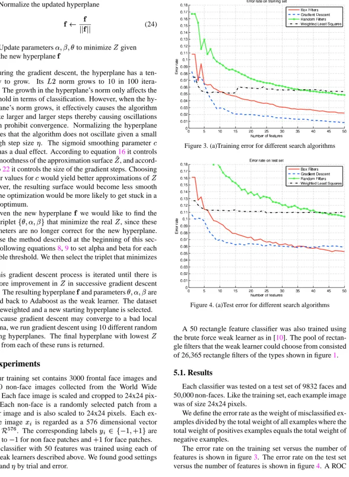
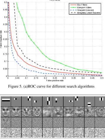
Each classifier was tested on a test set of 9832 faces and 50,000 non-faces. Like the training set, each example image was of size 24x24 pixels.
We define the error rate as the weight of misclassified ex-amples divided by the total weight of all exex-amples where the total weight of positives examples equals the total weight of negative examples.
The error rate on the training set versus the number of features is shown in figure3. The error rate on the test set versus the number of features is shown in figure4. A ROC 5
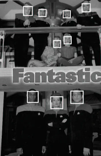
curve plotting false positive rate versus false negative rate on the test set is shown in figure5. For the ROC curves, only 10 features were used in each classifier. This is because on a typical face detector cascade, the average number of features computed per patch is less than 10 so the first 10 features really determine the speed of the classifier.
As expected, the brute force weak learner that uses a ran-dom sample of hyperplanes, has low accuracy and is signif-icantly worse than the rectangle feature classifier.
WLS has fairly low error after the first feature, how-ever, it quickly falls behind the rectangle feature classifier as more features are selected. We suspect that the main reason for this behavior is the squared penalty term that penalizes correct detections with high margin.
The gradient descent weak learner does achieve a sig-nificant improvement over the rectangle feature classifier at least until about the 30th feature. In terms of their ROC curves, the thresholded hyperplanes from the gradient de-scent weak learner achieve an equal error rate (where the false positive rate equals the false negative rate) of about 6.8 % while the rectangle features have an equal error rate of about 9.4 %. The main effect of this improved accuracy in the beginning stages of a cascade are on the average num-ber of features computed per image patch. For example the gradient descent based classifier after one weak classifier has about the same error on the test set as the rectangle fea-ture classifier after about 7 weak classifiers. The rectangle feature classifier takes about 23 weak classifiers to acheive the same error rate as the gradient descent based classifier after only 10 hyperplanes. In practice, this means that many fewer thresholded hyperplanes are needed to achieve the same error rate as the rectangle features. This leads to a significant reduction in the average number of features com-puted per patch in a cascaded detector.
It is also interesting to visualize the first few hyperplanes selected by each of the weak learners and the first few rect-angle filters selected. The first few hyperplanes chosen by the gradient descent weak learner look distinctly face-like as shown in figure6. The hyperplane chosen by weighted least squares has very little face-like structure which also helps explain why it generalizes more poorly.
5.2. Hardware oriented hybrid detectors
In practice most of the computation of a cascaded face detector is spent on the first 10 or so features. Therefore, us-ing on average less features at the beginnus-ing of the cascade while achieving the same error rate will greatly increase the speed of the detector. This is what is exactly what we get by using the gradient descent based detector presented here when concatenated to an existing rectangle filter based de-tector. Because general dot products can be very fast in hardware, these results have greatest importance for hard-ware implementations of face detectors which are becoming
Figure 5. (a)ROC curve for different search algorithms
Figure 6. First 10 hyperplanes chosen by the different algorithms. Each row represents a different selection algorithm. The features are sorted by selection order from left to right. (row 1)Viola and Jones box-filters (row 2) Gradient descent (row 3) Weighted least squares ( row 4) Random hyperplanes
quite common.
To build a full face detector, many more weak classifiers would have to be learned than just the first 50. The learning process also requires some form of resampling to generate more difficult non-face patches. Instead of training a full gradient descent based detector, we created a hybrid detec-tor. This was done by adding the first 10 thresholded hyper-planes learned using the gradient descent to the beginning of an existing rectangle filter based detector. The original box filter based detector has 1520 rectangle features. Thus, the hybrid detector has 1530 features. We tested the average number of weak classifiers evaluated per candidate patch for such a hybrid detector. On the MIT+CMU test set [9,7], which has 130 images and 507 faces, the box filter based de-tector at aëëì detection rate and a 1/1,014,170 false posi-tive rate evaluates on average 9.9 features per patch. The hy-brid detector at aëGë.ì detection rate and a 1/1,029,310 false positive rate evaluates on average 8.0 features per patch. Therefore, for approximately the same point on the ROC curve the hybrid detector yields almost a« Ç
ì speed up in terms of the number of features evaluated per patch. Some
Figure 7. Example of detections on a low contrast image
detection results for the hybrid detector on difficult images from the MIT+CMU test set are shown in figures7and8. These show detections on a low contrast image an image with a variety of different types of faces and slightly differ-ent poses.
6. Conclusions
Haar-like features are very difficult to improve on for general purpose computers in terms of their ratio of clas-sification accuracy over computational cost. However, for specialized hardware in which dot products are very fast, the costs change, and more powerful features such as real hyperplanes (dot products) can be just as cheap to compute. For such cases, we have shown that real hyperplane fea-tures can lead to significant improvements over Haar-like features. Thus, the main contributions of this paper are a new gradient descent weak learning algorithm for unre-stricted thresholded hyperplanes and the demonstration that such weak classifiers can lead to a significant speed-up in a cascaded face detector in terms of number of features com-puted per patch.
References
[1] Y. Freund and R. E. Schapire. A decision-theoretic gener-alization of on-line learning and an application to boosting. In Computational Learning Theory: Eurocolt ’95, pages 23– 37. Springer-Verlag, 1995. 2
[2] J. Friedman. Greedy function approximation: a gradient boosting machine, 1999. 4
[3] C. Huang, H. Ai, Y. Li, and S. Lao. Learning sparse features in granular space for multi-view face detection. In Proc. of
IEEE International conference on Automatic Face and Ges-ture Recognition, Southampton, UK, April 2006. 2
[4] S. Li and Z. Zhang. Floatboost learning and statistical face detection, 2004. 2
Figure 8. Example of detections on a wide variety of faces
[5] R. Lienhart and J. Maydt. An extended set of haar-like fea-tures for rapid object detection. In International Conference
on Image Processing, pages I: 900–903, 2002. 1,2
[6] C. Liu and H. Shum. Kullback-leibler boosting. In
Proceed-ings of the IEEE Conference on Computer Vision and Pattern Recognition, pages 587–594, 2003. 1
[7] H. Rowley, S. Baluja, and T. Kanade. Neural network-based face detection. In IEEE Patt. Anal. Mach. Intell., volume 20, pages 22–38, 1998. 6
[8] R. Schapire and Y. Singer. Improving boosting algo-rithms using confidence-rated predictions. Machine
Learn-ing, 37(3), 1999. 2,3
[9] K. Sung and T. Poggio. Example-based learning for view-based face detection. In IEEE Patt. Anal. Mach. Intell., vol-ume 20, pages 39–51, 1998. 6
[10] P. Viola and M. Jones. Robust real-time face detection. Int.
J. Computer Vision, 57:137–154, 2004. 1,2,5