CMM hardware error simulation for uncertainty
evaluation
Nick Van Gestel, Philip Bleys, Jean-Pierre Kruth
K.U.Leuven, department of Mechanical Engineering, Celestijnenlaan 300b, 3001 Heverlee, Belgium
Abstract
Uncertainty evaluation software based on Monte Carlo simulations is very useful for coordinate measurement machines (CMMs). These Monte Carlo methods use so-called virtual CMMs to simulate CMM measurement errors. Based on the simulated errors measurement uncertainties can be determined. This paper shows how CMM hardware errors can be modelled in a simple and straightforward way. It considers CMM geometric errors as well as probe and articulating probe head errors. A key element of the presented method is the selection of representative virtual CMMs based on a virtual ISO 10360-2 acceptance test. The method has been implemented in own developed uncertainty evaluation software but can also be used in other software. Re-sults show that very reliable uncertainty statements are obtained with this method.
Keywords: CMM, virtual CMM, geometric errors, measurement uncertainty, uncertainty evaluation software, Monte Carlo
1. Introduction
Knowing the measurement uncertainty is indispensable when evaluating conformance of products to tolerances [1]. Neglecting measurement uncer-tainty can result in false rejection or false acceptance of products. However, when using coordinate measuring machines (CMMs) the measurement un-certainty is often not taken into account because it is difficult to determine. Measurement uncertainty determination for coordinate measuring ma-chines is difficult because of the many uncertainty contributors (CMM hard-ware errors, temperature, measurement strategy, . . . ) that are involved [2]. Measurement uncertainty determination with uncertainty evaluation soft-ware (UES) based on Monte Carlo simulations is a valuable alternative to conventional uncertainty calculation methods, that are based on analytical propagation of standard uncertainties [3]. Monte Carlo methods can cope much better with the complexity of CMM measurements.
Several authors have already successfully proven the usefulness of Monte Carlo methods to calculate CMM measurement uncertainties; these methods make use of Virtual CMMs that should simulate realistic CMM behaviour [4, 5, 6, 7]. Existing methods usually require a time consuming calibration procedure and do not take specific uncertainty contributors, like Abbe-errors and squareness errors, completely into account [8]. The method that is pro-posed in this paper takes into account the influence of Abbe-distances and squareness errors on the measurement uncertainty while it ‘only’ requires a valid ISO 10360-2 specification of the CMM to select representative virtual CMMs.
2. Hardware uncertainty contributors
Although they are not the only measurement uncertainty contributors, CMM hardware errors are often regarded as a very important source of mea-surement uncertainty. For a conventional CMM, hardware errors can be divided into two main categories:
Geometric errors Due to mechanical imperfections of guideways and
car-riages of a Cartesian CMM, linear motions along the axes will not be perfectly straight. These error motions are called geometric errors of the CMM.
Probing system and probe head errors The probing system, possibly
mounted on an indexable probing head, will usually have a notable influence on the measurement uncertainty.
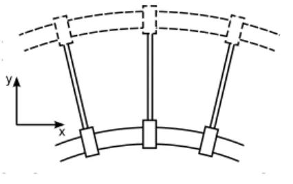
It should be clear that CMM hardware uncertainties can never be treated without considering environmental influences. Environmental conditions (like e.g. temperature) will have an important influence on hardware uncertainties [9, 10]. The geometric errors of the 3 axes of a conventional CMM are char-acterized by 6 error motions: 3 linear and 3 angular error motions, illustrated in Fig. 1 for the z-axis [11].
In this paper the conventions according to ISO 230-1 are used; further in this text often lower case letters are used for reasons of readability (e.g.
exx instead of EXX). Besides the 6 errors of motion for each axis, usually three additional squareness errors are defined because the three axes are not perfectly perpendicular to each other. This means that the geometric errors
EXZ: Straightness error motion of thez-axis inxdirection EYZ: Straightness error motion of thez-axis inydirection EZZ: Positioning error of thez-axis
EAZ: Tilt error motion of thez-axis aroundx(pitch) EBZ: Tilt error motion of thez-axis aroundy (yaw) ECZ: Roll error motion of thez-axis
Figure 1: Error components for a straight line motion along the z-axis. Adapted from [11].
of a CMM can be described by 21 (3×6 + 3) parametric errors, if the rigid body assumption is valid.
3. Kinematic model of CMM-measurement
Most conventional CMMs can be modelled as a kinematic chain of 4 rigid bodies connected by 3 prismatic joints. To each of the four rigid bodies a frame can be assigned. The kinematic chain of the CMM at the laboratory of K.U.Leuven (Coord3 MC16) is depicted in Fig. 2; the frames are assigned as follows:
• Frame {0} is connected to the fixed CMM structure (granite table), and corresponds to the machine coordinate system (MCS).
• Frame {1} is connected to the x-carriage (portal structure).
• Frame {2} is connected to the y-carriage (saddle).
• Frame {3} is connected to the z-ram.
The motion of the frames relative to each other, through the prismatic joints, can be described by homogeneous transformation matrices. In case of error-free prismatic joints, the homogeneous transformation matrix describ-ing the pose of frame{1}with respect to frame{0}, expressed in frame {0}, is as follows: 1 0T = 1 0 0 0x0x+xenc 0 1 0 0y0x 0 0 1 0z0x 0 0 0 1 (1)
Figure 2: The kinematic chain of the Coord3 MC16 CMM.
This homogeneous transformation matrix is describing a simple transla-tion. xenc represents the value read from the x-scale (linear encoder of the
x-scale). (0x0x,0y0x,0z0x) corresponds to the beginning (home position) of
the x-scale, expressed in frame{0}. This means that the origin of frame{1} is connected to the reference point of the scale reading unit mounted on the
x-carriage.
If the error motions of thex-carriage are taken into account, Eq. 1 extends to: 1 0T =
1 −ecx ebx 0x0x+xenc+exx
ecx 1 −eax 0y0x+eyx
−ebx eax 1 0z0x+ezx
0 0 0 1 (2)
It should be noticed that the error motions e∗x (∗ is used as wildcard character) of Eq. 2 are no single values but that they depend on the position of the x-axis; this means that they are function ofxenc. Instead of e∗x(xenc) the short notation e∗x is used. The short notation is also used to refer to the y- and z-error motions.
The motion of the y-carriage (frame {2}) with respect to the x-carriage and the motion of the z-ram (frame {3}) with respect to the y-carriage can be described by two analogue transformation matrices 2
1T and 32T.
Frame {3} is not suited to be used as reference frame since its position has no practical value. It is better to use the end of the z-ram as reference frame (frame{m} in Fig. 2). This position is called theprobe head mounting point, because that is the position where the probe head is mounted. Since this is a position on thez-ram, the transformation matrix describing the pose of frame {m} with respect to frame{3} represents a simple translation:
m 3 T = 1 0 0 3x0m 0 1 0 3y0m 0 0 1 3z0m 0 0 0 1 (3)
(3x0m,3y0m,3z0m) corresponds to the position the probe head mounting
point, expressed in frame {3}. Based on m
3 T, 32T, 21T and 10T, the homogeneous transformation matrix
describing the pose of frame{m}with respect to frame{0}can be calculated:
m
Calculating this set of matrix multiplications, and neglecting second order effects (e∗∗ ·e∗∗ ≈0) gives following extensive matrix:
m 0 T= m 0 R 0p0,m 01×3 1 (5) with m 0 R=
1 −ecz−ecy−ecx ebz+eby+ebx ecx+ecy+ecz 1 −eaz−eay−eax −ebx−eby−ebz eax+eay+eaz 1
(6) and 0p0,m =
xenc+x0x+x0y+x0z+x0m+exx+exy+exz −ecz y0m+ebx z0y+ebz z0m−ecx(y0y+yenc)
−(ecy+ecx)(y0m+y0z) +(eby+ebx)(z0m+zenc+z0z)
yenc+y0x+y0y+y0z+y0m+eyx+eyy+eyz +ecz x0m+ecx x0y−eax z0y−eaz z0m
+(ecx+ecy)(x0m+x0z) −(eay+eax)(z0m+zenc+z0z)
zenc+z0x+z0y+z0z+z0m+ezx+ezy+ezz −ebz x0m+eaz y0m−ebx x0y+eax(y0y+yenc)
−(ebx+eby)(x0m+x0z) +(eax+eay)(x0m+y0m+y0z) (7) m
0 Rrepresents the total angular error of thez-ram expressed with respect
to frame {0}. It can be calculated as the sum of the angular errors of all separate axes. 0p0,m represents the position of the probe head mounting
point. Errors on this position depend on the positioning and straightness errors of the different axes, but also on the angular error motions of these
axes. These latter errors are the so called ‘Abbe errors’ and depend on the position of the probe head mounting point with respect to the different scales. The closer to the scales, the smaller the effect of these errors [12]. In Eq. 7 the parameters ∗0∗ are no longer accompanied by the leading subscripts (as in Eq. 2 to 3) for reasons of readability.
The position of the probe head mounting point is usually not the position of interest when using the CMM. For tactile sensors the center of the stylus tip is determined as reference. The position of this reference point is important to calculate the effect of the angular errors. The position of the probe tip, with respect to the probe head mounting point can be expressed by following homogeneous transformation matrix:
p mT = 1 0 0 mxp 0 1 0 myp 0 0 1 mzp 0 0 0 1 (8) p
mT does not include errors due to the probing system. The modelling of probing errors is discussed in section 8. To calculate the effect of CMM geometric errors on the probe reference point (xp, yp, xp), only its nominal position is needed. The transformation matrix describing the complete kine-matic chain of the CMM is then calculated as:
p 0T =m0 T pmT = p 0R 0p0,p 01×3 1 (9) with p 0R=m0 R (10)
and 0p0,p =m0 R mxp myp mzp +0p 0,m (11)
One could wonder why squareness errors are not included in all equations above; the equations only show 18 instead of 21 error components. In the model presented above it is assumed that squareness errors are included in the straightness errors. When measuring geometric errors, one usually considers straightness errors and squareness errors as two different error components because they are usually measured in different setups. However, the square-ness error can be added to the straightsquare-ness error by adding the squaresquare-ness value (expressed as µm/m) as a linear component to the straightness error.
4. Need for scale positions in the kinematic CMM model
Vector0p0,m(Eq. 7) is quite complicated because the real positions of the scales (∗0∗) are taken into account. If the scales are treated as coincident with the axes of the MCS (frame {0}) all ∗0∗ values are zero, and Eq. 7 simplifies to: 0p0,m =
xenc+exx+exy+exz−yencecx+zenc(ebx+eby) yenc+eyx+eyy+eyz−zenc(eax+eay)
zenc+ezx+ezy+ezz+yenceax
(12)
This equation looks more like results obtained by other authors [13, 14, 15]. One could wonder why the position of the scales is usually not taken into account when modelling CMM geometric errors. Most articles describing geometric errors deal with compensating geometric errors of a CMM, or other
Figure 3: Two axes configurations that describe the same error motion.
machine tools; it is the purpose to compensate the systematic errors as good as possible and not to model the remaining errors after compensation. The position of the scales does not matter for error compensation. To illustrate that Fig. 3 shows a simplified example for the compensation of an error motion of one axis (x-axis).
Fig. 3 shows an axis that is bent, resulting in a yaw error ecx. If the positioning errors exx are considered to be zero, the errors will rise with increasing y-value, as illustrated in Fig. 3. The measured geometric errors can be used to compensate for the error motions. The geometric errors exx,
ecxcould be measured with a laser interferometer that is positioned as close as possible to the x-guideway (y = 0). However, if the laser interferometer is positioned further away from the x-guideway (y =y1) positive positioning
errors will be measured by the laser interferometer, while the measured yaw errors will be independent of the position of the laser interferometer. One can imagine a virtual guideway at y = y1 with a positive positioning error
and the same yaw error (dotted guideway in Fig. 3).
The measured positioning error will be influenced by angular errors, if the measurement is not performed in line with the scale of the guideway. But the position of the scales in the CMM model is not important for the
compensation of systematic error motions. It does not matter whether or not the measured positional and linear deviations are also influenced by angular errors of the guideway. As long as the geometric errors do not change the calculated compensations will be the same.
However, in order to determine the measurement uncertainty (after cali-bration of the CMM) the position of the axis is really important. If there are uncompensated yaw-errors in the example above, they will hardly influence measurements close to the x-scale (y≈0) while they can have an important influence for measurements further away from the x-scale (y �0).
If one wants the CMM model to reflect the ‘Abbe errors’ correctly, the position of the scales should be integrated in the CMM model. Measurement positions further from the scales will have larger measurement uncertainties than positions close to the scales. This should be integrated in the uncer-tainty calculations. Therefore it is important that the positions of the scales are modelled correctly.
5. Simulating geometric error components
Eq. 7 and 11 can be used to simulate errors on the position of theprobe head mounting point and theprobe tip position. In order to do so, information about the configuration of the CMM (position of the scales) is needed as well as information about the geometric errors of the CMM. Information about the configuration of the CMM can be easily obtained (see further in section 6). Obtaining information about the geometric errors of the CMM is not so obvious. Measuring the geometric errors of a CMM can be done in several ways: e.g. by laser interferometer and electronic levels or by means of
multilateration techniques [16]. Regardless of the used method, measuring all 21 geometric errors is very time consuming. Yet, knowing the true geometric errors is not essential for uncertainty modelling :
• If the geometric errors are known, they should be compensated. The concept that known systematic errors should be compensated, and not included in the measurement uncertainty, is one of the basic principles of the GUM [17].
• Measured geometric errors can seldom be considered as invariable. In a limited time period, geometric errors often stay quite constant but when the geometric errors are remeasured after a longer period, they can look very different due to (thermal) drift of the machine.
• For measurement uncertainty determination it is important that the obtained measurement uncertainties are reliable. The actual values of the the true geometric errors do not matter, as long as the calculated measurement uncertainties are reliable. The actual values of the true geometric errors are needed for calibration, but not for measurement uncertainty determination.
The central idea of the proposed approach is that it is impossible and unnecessary to know the true geometric errors of a CMM for uncertainty calculations. This does not mean that it is unnecessary to be able to simulate
realistic geometric errors. Realistic geometric errors will be necessary to simulate realistic measurement errors in order to obtain reliable measurement uncertainties.
0 500 1000 1500 2000 −6 −4 −2 0 2 4 X [mm] Error [ µ m]
Positioning error X−axis (EXX)
0 500 1000 1500 2000 −6 −4 −2 0 2 4 X [mm] Error [ µ m]
Straightness error motion of X in Y direction (EYX)
0 500 1000 1500 2000 −6 −4 −2 0 2 4 X [mm] Error [ µ m]
Straightness error motion of X in Z direction (EZX)
0 200 400 600 800 1000 −6 −4 −2 0 2 4 Y [mm] Error [ µ m]
Straightness error motion of Y in X direction (EXY)
0 200 400 600 800 1000 −6 −4 −2 0 2 4 Y [mm] Error [ µ m]
Positioning error Y−axis (EYY)
0 200 400 600 800 1000 −6 −4 −2 0 2 4 Y [mm] Error [ µ m]
Straightness error motion of Y in Z direction (EZY)
−800 −600 −400 −200 0 −6 −4 −2 0 2 4 Z [mm] Error [ µ m]
Straightness error motion of Z in X direction (EXZ)
−800 −600 −400 −200 0 −6 −4 −2 0 2 4 Z [mm] Error [ µ m]
Straightness error motion of Z in Y direction (EYZ)
−800 −600 −400 −200 0 −6 −4 −2 0 2 4 Z [mm] Error [ µ m]
Positioning error Z−axis (EZZ)
0 500 1000 1500 2000 −5 0 5 X [mm] Error [ µ m/m]
Roll error motion X−axis (EAX)
0 500 1000 1500 2000 −5 0 5 X [mm] Error [ µ m/m]
Pitch error motion of X (EBX)
0 500 1000 1500 2000 −5 0 5 X [mm] Error [ µ m/m]
Yaw error motion of X (ECX)
0 200 400 600 800 1000 −5 0 5 Y [mm] Error [ µ m/m]
Pitch error motion of Y (EAY)
0 200 400 600 800 1000 −5 0 5 Y [mm] Error [ µ m/m]
Roll error motion Y−axis (EBY)
0 200 400 600 800 1000 −5 0 5 Y [mm] Error [ µ m/m]
Yaw error motion of Y (ECY)
−800 −600 −400 −200 0 −5 0 5 Z [mm] Error [ µ m/m]
Tilt error motion of Z around X (EAZ)
−800 −600 −400 −200 0 −5 0 5 Z [mm] Error [ µ m/m]
Tilt error motion of Z around Y (EBZ)
−800 −600 −400 −200 0 −5 0 5 Z [mm] Error [ µ m/m]
Roll error motion Z−axis (ECZ)
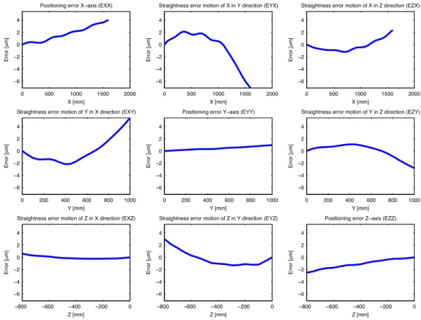
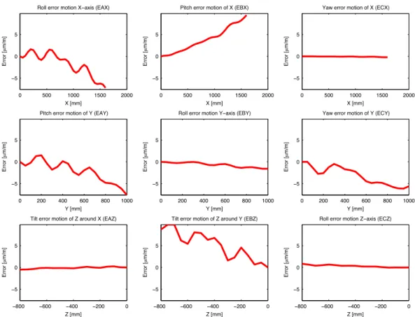
Based on in-house experience on other machine tools and examples from literature [18, 14, 19] it can be stated that geometric errors are dominated by linear and curvature components. Simulated geometric errors should have similar properties as measured geometric errors. Linear and curvature com-ponents of a geometric error can be described by a linear and quadratic function. Apart from these components, geometric errors usually also show some more random variations that can be modelled by adding some ran-dom harmonics. The function for modelling geometric errors (e(x)) looks as follows: e(x) = sx+c(2x2−1) + N � n=1 ancos(nπx+φn) (13)
for x∈[−1,1] and with
s+c+ N
�
n=1
an= 1 (14)
The values of parameters s and c will determine the importance of re-spectively the linear and curvature component of the geometric error. N de-termines the maximum harmonic order, expressed in undulations per length (UPL). The simulation of geometric errors by means of Fourier series has al-ready been applied in Monte Carlo simulations for machine tools and CMMs [20, 21].
The values foran can be specified by the user but are usually determined randomly. A geometric error will be represented by a vector e, obtained by evaluating Eq. 13 for a discrete set of values for x. It describes a geometric error (e.g. exx) over the length of the respective axis. The first value of the error vectore is put at zero because geometric errors are zero by definition at the origin of the scale. This zeroing is implemented by subtracting the first
value from the complete error vector. Additionally the maximum absolute value of the error vector e is rescaled to 1 by dividing the vector by its maximum absolute value.
The advantage of having this rescaled error vector is that it can be rescaled to an error vector of whatever magnitude, just by multiplying it by a given error value etot. This will be the largest value of the geometric error over the total range of the axis:
e←etote (15)
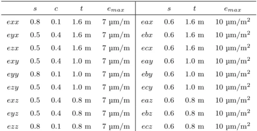
A realistic value foretot should be chosen. In reality the geometric error will be strongly dependent on the length. The longer the travel of the axis, the larger the error can be. Therefore it would be logical to choose these values proportional to the length of the axis. One can choose these values based on the ISO 10360-2 specification of the CMM. E.g. a CMM with a specification of 5 µm + 5 µm/m will not show positioning errors of 20 µm/m. Based on the performance specification one can roughly estimate the maximum possible value for the geometric erroremaxthat represents the maximum error value per travel length. emax is expressed in µm/m for positional and linear deviations and is expressed in µm/m2 for angular deviations. Once e
max is known, etot can be determined by multiplyingemax with the total travel t of the axis (in meter). Not every simulated geometric error component needs to have the maximum value; errors will often be smaller. The sign of the errors can also be positive or negative. That is why etot is determined by additionally multiplying emax with a random value, ranging between −1 and 1:
s c t emax s t emax exx 0.8 0.1 1.6 m 7µm/m eax 0.6 1.6 m 10µm/m2 eyx 0.5 0.4 1.6 m 7µm/m ebx 0.6 1.6 m 10µm/m2 ezx 0.5 0.4 1.6 m 7µm/m ecx 0.6 1.6 m 10µm/m2 exy 0.5 0.4 1.0 m 7µm/m eay 0.6 1.0 m 10µm/m2 eyy 0.8 0.1 1.0 m 7µm/m eby 0.6 1.0 m 10µm/m2 ezy 0.5 0.4 1.0 m 7µm/m ecy 0.6 1.0 m 10µm/m2 exz 0.5 0.4 0.8 m 7µm/m eaz 0.6 0.8 m 10µm/m2 eyz 0.5 0.4 0.8 m 7µm/m ebz 0.6 0.8 m 10µm/m2 ezz 0.8 0.1 0.8 m 7µm/m ecz 0.6 0.8 m 10µm/m2
Table 1: Parameters used to simulate the geometric errors of figures 4 and 5.
Fig. 4 shows the simulated positioning and straightness errors for one virtual CMM. Fig. 5 shows the angular errors. Table 1 shows the parameter settings that were used to generate the geometric errors,N was always taken equal to 7.
All geometric errors are generated independently from each other, so there will be no correlation between different geometric errors. This is a simplifica-tion of reality; in practice geometric errors will be correlated due to thermal influences and the fact that angular deviations are caused by the straightness deviation of the axes.
6. Calculating error states of virtual CMMs
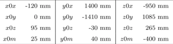
Once all geometric errors are simulated, Eq. 7 can be used to calculate the resulting errors on the probe head mounting point in the measurement space of the CMM. The resulting errors over the whole measurement space of the CMM are called theerror state. To calculate this error state, information about the position of the axes is needed. Table 2 shows the values of the axes position parameters used to calculate the error state for the Coord3 MC16
x0x -120 mm y0x 1400 mm z0x -950 mm
x0y 0 mm y0y -1410 mm z0y 1085 mm
x0z 95 mm y0z -30 mm z0z 265 mm
x0m 25 mm y0m 40 mm z0m -400 mm
Table 2: Axes position parameters used to simulate the error state.
CMM.
From Eq. (7) the relationship between thenominal (error free) position of probe head mounting point, expressed in the MCS, and the values read from the scales xenc, yenc, zenc can be derived:
0xm =xenc+x0x+x0y+x0z+x0m
0ym =yenc+y0x+y0y+y0z+y0m
0ym =zenc+z0x+z0y+z0z+z0m
(17)
When the home position of the scales (xenc, yenc, zenc = 0) corresponds to the nominal home position of the probe head mounting point expressed in the MCS (0xm,0ym,0zm = 0), the sum of all axes translations should be zero. The values of Table 2 meet this requirement. If the axes positions are known and the 18 geometric errors are simulated, Eq. 7 or Eq. 11 can be used to calculate the errors on the position of the probe head or respectively the center of the probing tip.
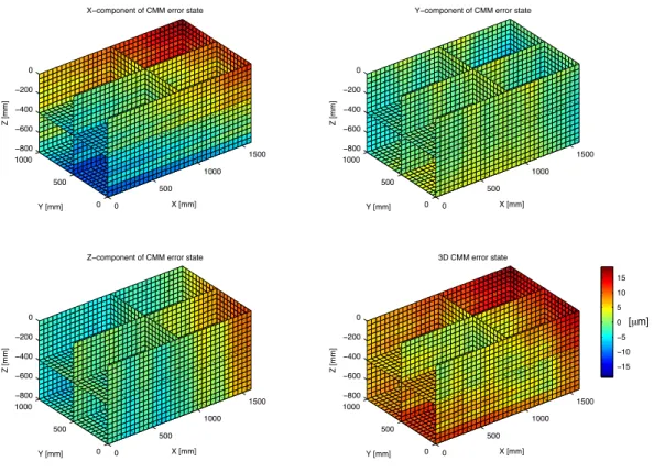
Fig. 6 shows the calculated error state for the axes position parameters of Table 2 and the geometric errors represented in figures 4 and 5. These figures represent the x, y, and z-errors of a virtual CMM with the same measurement volume and the same configuration of its axes as the actual CMM. All errors are zero for (0xm,0ym,0zm) = (0,0,0) since all geometric
bottom-0 500 1000 1500 0 500 1000 −800 −600 −400 −200 0 X [mm] X−component of CMM error state
Y [mm] Z [mm] 0 500 1000 1500 0 500 1000 −800 −600 −400 −200 0 X [mm] Y−component of CMM error state
Y [mm] Z [mm] 0 500 1000 1500 0 500 1000 −800 −600 −400 −200 0 X [mm] Z−component of CMM error state
Y [mm] Z [mm] 0 500 1000 1500 0 500 1000 −800 −600 −400 −200 0 X [mm] 3D CMM error state Y [mm] Z [mm] −15 −10 −5 0 5 10 15 [µm]
Figure 6: Simulated error state for a virtual CMM (‘intersection’-planes are used for better visualisation of the errors).
right figure, representing the 3D-error state, indicates the total error that is calculated as follows:
errd=�errx2+erry2+errz2 (18)
Although the positions close to the origin show small errors, and positions further from the origin mostly show larger errors, this does not mean that the CMM will measure more accurately in zones that show small errors. The error variations are important for the error on the measurement result, not the magnitude of the error.
7. Selecting representative virtual CMMs
The simulated errors should not be the same as the errors of the actual CMM but should nevertheless be representative for this CMM. One could check if the magnitude of the errors of the actual CMM corresponds to the magnitude of the simulated errors by comparing an actually measured ref-erence artefact (e.g. gauge block) with a simulated measurement of that object. Yet performing actual measurements can take a lot of time.
It is not necessary to make use of actual measurements if one uses the ISO 10360-2 performance specification for length measurements. If there is a valid ISO 10360-2 specification, one knows that every actual length mea-surement (according to ISO 10360-2) will have an error lower than the given MPE (maximum permissible error). This information can be used to check if simulated measurements of the virtual CMM fall within these limit. Every virtual CMM will be subjected to a virtual ISO 10360-2 test. This test is used to check if the virtual CMM is representative for the true CMM.
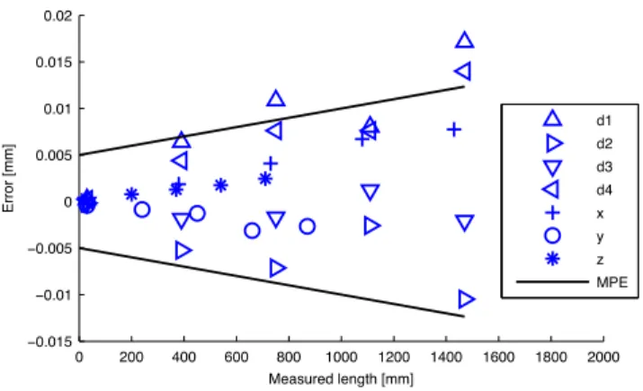
0 200 400 600 800 1000 1200 1400 1600 1800 2000 −0.015 −0.01 −0.005 0 0.005 0.01 0.015 0.02 Measured length [mm] Error [mm] d1 d2 d3 d4 x y z MPE
Figure 7: ISO 10360-2 test for the virtual CMM of Fig. 6.
According to ISO 10360-2 a set of five material standards of size (step gauge or gauge blocks) needs to be measured in seven different orientations on the CMM, and each measurement is repeated three times [22]. The short-est material of size should be smaller than 30 mm, the longshort-est should be longer than 66% of the largest spatial diagonal of the measuring volume of the CMM. For each of the 105 measurements, the error on size E is calcu-lated. All errors are plotted on a graph in function of the measured length. Fig. 7 shows the graph of such a simulated measurement for the virtual CMM represented in Fig. 6. Measurements labelled as d1, d2, d3 and d4 represent measurement errors along the four diagonals; measurement labelled x,y and
z represent measurement errors along the respective axes. Since no random geometric errors or probing errors are included, performing the same mea-surement three times yields three times the same result. Therefore only 35 virtual measurements are done rather than the 105 (35×3) measurements required by ISO 10360-2.
the MPE-limits of the actual CMM (5 µm ± 5 µm/m). But the errors are also not extremely large compared to the MPE. Other virtual CMMs, cre-ated with the same parameters showed errors that were all lower than the specified MPE. This means that the chosen parameters for the simulated geo-metric errorsemax are satisfying. In order to measure how well the simulated CMM corresponds to the performance specification of the actual CMM, a performance indicator v for each virtual CMM is calculated:
v =min����� mpel errl � � � � �
for all 35 measured lengths (19)
where errl represents the virtually measured error on a given length and mpel represents the MPE for that length. If the performance indicator v is lower than 1, the virtual CMM has not passed the ISO 10360-2 test and is considered as unsuited for simulation purposes. If the value of v is higher than 2, which means that no simulated measurement error is larger than half its MPE, the errors are considered as too small. In this case the virtual CMM is also not representative for the actual CMM, because its errors are too low. If virtual CMMs are used for error simulation in a Monte Carlo method, multiple virtual CMMs will be needed. It is impossible to choose the pa-rameters for the geometric errors in such way that all simulated CMMs have values of v between 1 and 2, because the generated geometric errors have a large degree of randomness. If too much (e.g. more than 50%) virtual CMMs fail because their errors are too low or too high, the parameters for the gen-eration of the geometric errors are probably wrongly selected and should be adapted.
Figure 8: Representation of an articulating system with two angles (Renishaw PH10M), adapted from [23].
8. Modelling probing system errors
8.1. Modelling the nominal position of the probe tip
In order to complete the kinematic model of the CMM, the position of the probe tip with respect to the probe head mounting point is needed (see Eq. 11). Therefore the dimensions and the configuration of the probing sys-tem have to be known. Fig. 8 shows a drawing of the articulating probe head, equipped with probe and stylus, used on the Coord3 CMM. The nomi-nal position of the probe tip with respect to frame{m}(mxp,myp,mzp) can be easily expressed in function of theAand B angles (θA, θB) of the articulating probe head system:
mxp myp mzp 1 = r mR mpm,r 01×3 1 rxp ryp rzp 1 (20)
with r mR=
cos(θA) cos(θB) −sin(θB) −sin(θA) cos(θB) cos(θA) sin(θB) cos(θB) −sin(θA) sin(θB)
sin(θA) 0 cos(θA) (21) and mpm,r = mxr myr mzr (22)
(rxp,ryp,rzp) represents the position of the center of the stylus tip, ex-pressed in frame {r}. The origin of frame {r} corresponds to the center of rotation of the articulating probe head. This frame is connected to the last linkage of the articulating probe head (linkage to which the probe is mounted); this means that the position of the probe tip with respect to frame {r} does not change with changing A or B angle. r
mR is a rotation matrix representing the A and B rotation of the articulating probe head. This matrix is valid for the mounting configuration of the PH10M probe head on the Coord3 CMM. For other mounting configurations, matrix r
mR will look slightly different. mpm,r represents the position of the center point of the articulating probe head, with respect to the probe head mounting point. This is the intersection of the A-axis and B-axis and is usually only offset in negativez-direction with respect to the probe head mounting point: (mxr,myr,mzr) = (0,0,−lr) (23) For straight styli the nominal center position of the stylus tip (rxp,ryp,rzp) is usually only offset in negative z-direction over a length lp:
In this specific situation Eq. 20 results in: mxp myp mzp = sin(θA) cos(θB)lp sin(θA) sin(θB)lp −lr−cos(θA)lp (25)
These calculated nominal positions of the center of the stylus tip can be used in Eq. 11 to calculate the errors on the center point of the probe tip due to the geometric errors of the CMM. Information about the position of the probe tip is needed to know the actual Abbe distances to the different axes. Errors of the articulating probe head and probe can be modelled separately and added to the probe tip errors caused by geometric errors.
8.2. Modelling errors of the articulating probe head
The repeatability of the different angular positions of the articulating probe head is very good. The relative position of the probe tip can be calibrated before the start of the measurement. Once calibrated, all available probe configurations can be used with a very good repeatability, but the introduced errors can not be neglected. The influence of angular deviations from the nominal positions on the probe position can be obtained from Eq. 25. The angular errors errθ
A anderrθB are considered as the only relevant errors for the articulating probe head. This is a simplification of reality, since the real rotations around the A-axis as well as the B-axis exhibit three linear and three angular errors.
From manufacturer’s specifications an approximating value of 0.83�� for
the standard deviations of the angular errors errθ
A and errθB can be derived [23]. This value, verified by tests, is used to model probe position errors due
to the articulating probe head. These errors stay the same as long as the probe orientation is not changed; so in that case they can be considered as a kind of systematic errors. Errors of the articulating probe head will have no influence on the hardware uncertainties if only one probe configuration is used during the measurement.
8.3. Modelling errors of the probe
Besides geometric errors and errors of the articulating probe head, there are also the errors of the probe itself that are part of the hardware uncertain-ties. For modelling probe errors in detail, a dedicated model of the probe is needed. Modelling probe errors can be very difficult due to the large number of parameters and settings that will influence the probe errors: measurement speed, contact force, stylus length, probe tip diameter . . . Because of these difficulties, a pragmatic solution was chosen. The probe errors are modelled as random errors defined by given standard deviations for three orthogo-nal directions: σ(err
rxp), σ(errryp), σ(errrzp). These values are determined by the user and can be derived from actual tests or from specifications (e.g. ISO 10360 specification MPEP for the probing error).
Considering probe errors as purely random errors does not comply with the real behaviour of most probing system: e.g. switching touch-trigger probes exhibit systematic errors due to the varying pretravel distance.
9. Verification of results
This paper described how virtual CMMs, that have similar performance and error behaviour as the actual CMM, can be modelled. Virtual CMMs
Figure 9: Gauge blocks measurement on the CMM.
can be used in Monte Carlo simulations to calculate measurement uncertain-ties; the measurement will be simulated multiple times by virtual CMMs and the dispersion on the results will be used to calculate the measurement uncertainty. More details about the uncertainty evaluation software that in-corporates the methods described in this paper, can be found in an earlier publication [24]. This section describes a test to check the validity of the CMM hardware error modelling.
An easy way to verify errors of a CMM is to measure a set of gauge blocks. A gauge block has a reference length with a very low calibration uncertainty. The calculated errors, obtained by subtracting the reference value from the value measured with the CMM, can be compared with the calculated measurement uncertainties. The reference value should be situated within the calculated uncertainty interval for the measurement.
To prove the validity of the integrated hardware error model, multiple measurements are done of gauge blocks with different lengths under different orientations and on different locations in the CMM measurement volume. Two reference lengths, a short one (S: 99.99978 mm (U = 0.12 µm, k = 2)) and a longer one (L: 499.99890 mm (U = 1.2 µm, k = 2)), are measured
under 7 different locations or orientations. Every gauge block is aligned (i.e. a part coordinate system is defined) before its length is measured. For every measurement the measurement error is compared with the calculated measurement uncertainty. The settings used to model the geometric errors of the virtual CMMs are taken from Table 1. A normally distributed random error was used for the probing error (with σ = 0.5 µm). 1000 Monte Carlo runs were executed using each time another virtual CMM. The results were used to calculate the 95% confidence limits. Following different measurement positions and orientations are used:
• x1: along thex-direction, close to the x-scale.
• x2: along thex-direction, large Abbe-offset in y-direction to x-scale.
• y1: along they-direction, close to they-scale.
• y2: along they-direction, large Abbe-offset inz-direction to y-scale.
• z1: along thez-direction.
• d1: along a diagonal parallel to thex-y-plane.
• d2: along a space diagonal.
The results of the measurements and the calculated uncertainties are given in Table 3. The upper and lower confidence limits (UCL and LCL) are given relative to the measured values. It is clear from the results that all calculated uncertainties cover the true value, if the nominal value of the gauge blocks is considered as true value (the results are also valid if the calibration uncertainty of the gauge blocks is taken into account). It can also
LCL Meas. UCL Result x1 S -0.0017 100.0005 0.0017 ✓ L -0.0040 499.9988 0.0042 ✓ x2 S -0.0028 99.9976 0.0026 ✓ L -0.0049 499.9958 0.0051 ✓ y1 S -0.0018 99.9998 0.0019 ✓ L -0.0044 499.9998 0.0045 ✓ y2 S -0.0027 99.9986 0.0033 ✓ L -0.0073 500.0022 0.0081 ✓ z1 S -0.0016 99.9986 0.0017 ✓ L -0.0034 500.0019 0.0035 ✓ d1 S -0.0023 100.0013 0.0025 ✓ L -0.0058 500.0039 0.0059 ✓ d2 S -0.0025 99.9981 0.0024 ✓ L -0.0063 499.9974 0.0064 ✓
be seen that the calculated uncertainties take into account the effect of size (the uncertainties for the longer gauge block are systematically larger) and the effect of Abbe-errors (the measurements with larger Abbe-offsets result in larger uncertainties). These results confirm that the methods to model hardware uncertainties, described in this paper, result in reliable uncertainty statements.
10. Conclusions
This paper discussed the modelling of CMM hardware errors. Modelled hardware errors can be used for uncertainty evaluation of CMM measure-ments. To model the varying measurement accuracy of a CMM in its mea-surement volume, the position of the scales needs to be incorporated in the kinematic model of the CMM. This paper shows how this can be done.
The presented method uses simulated geometric error components. Based on the kinematic model of the CMM and 18 simulated geometric error com-ponents, the error state of a virtual CMM can be built. To check if a virtual CMM exhibits errors that are representative for the actual CMM, a virtual ISO 10360-2 test is performed. This yields a major advantage of the proposed method: no time consuming calibrations are necessary to built the virtual CMMs.
Besides the modelling of CMM geometric errors, this paper also describes the modelling of probe and probe head errors. The verification of the results showed that the calculated uncertainties based on this method are very reli-able.
11. References
[1] ISO 14253-1:1998, Geometrical Product Specifications (GPS) – Inspec-tion by measurement of workpieces and measuring equipment – Part 1: Decision rules for proving conformance or non-conformance with speci-fications, ISO, 1998.
[2] R. Wilhelm, R. Hocken, H. Schwenke, Task specific uncertainty in co-ordinate measurement, CIRP Annals-Manufacturing Technology 50 (2) (2001) 553–563.
[3] ISO/TS 15530-4:2008, Geometrical Product Specifications (GPS) – Co-ordinate measuring machines (CMM): Technique for determining the uncertainty of measurement – Part 4: Evaluating task-specific measure-ment uncertainty using simulation, ISO, 2008.
[4] A. Balsamo, M. Di Ciommo, R. Mugno, B. Rebaglia, E. Ricci, R. Grella, Evaluation of CMM uncertainty through Monte Carlo simulations, CIRP Annals-Manufacturing Technology 48 (1) (1999) 425–428.
[5] H. Schwenke, B. Siebert, F. W¨aldele, H. Kunzmann, Assessment of un-certainties in dimensional metrology by Monte Carlo simulation: pro-posal of a modular and visual software, CIRP Annals-Manufacturing Technology 49 (1) (2000) 395–398.
[6] B. van Dorp, H. Haitjema, F. Delbressine, R. Bergmans, P. Schellekens, Virtual CMM using Monte Carlo methods based on frequency content of the error signal, in: Proc. SPIE, Vol. 4401, 2001, p. 158.
[7] P. Ramu, J. Yague, R. Hocken, J. Miller, Development of a paramet-ric model and virtual machine to estimate task specific measurement uncertainty for a five axis multi sensor coordinate measuring machine, Precision Engineering 35 (2011) 431–439.
[8] J. Beaman, E. Morse, Experimental evaluation of software estimates of task specific measurement uncertainty for CMMs, Precision Engineering 34 (1) (2010) 28–33.
[9] J.P. Kruth, P. Vanherck, C. Van den Bergh, Compensation of static and transient thermal errors on CMMs, CIRP Ann. 50 (1) (2001) 377–380.
[10] J.P. Kruth, P. Vanherck, C. Van den Bergh, B. Schacht, Interaction between workpiece and CMM during geometrical quality control in non-standard thermal conditions, Precis. Eng. 26 (1) (2002) 93–98.
[11] ISO 230-1:1996, Test code for machine tools – Part 1: Geometric accu-racy of machines operating under no-load or finishing conditions, ISO, 1996.
[12] W. Knapp, E. Matthias, Test of the three-dimensional uncertainty of machine tools and measuring machines and its relation to the machine errors, CIRP Annals-Manufacturing Technology 32 (1) (1983) 459–464.
[13] G. Zhang, R. Veale, T. Charlton, B. Borchardt, R. Hocken, Er-ror compensation of coordinate measuring machines, CIRP Annals-Manufacturing Technology 34 (1) (1985) 445–448.
[14] P. Huang, J. Ni, On-line error compensation of coordinate measur-ing machines, International Journal of Machine Tools and Manufacture 35 (5) (1995) 725–738.
[15] J.P. Kruth, P. Vanherck, L. De Jonge, Self-calibration method and soft-ware error correction for three-dimensional coordinate measuring ma-chines using artefact measurements, Measurement 14 (2) (1994) 157– 167.
[16] H. Schwenke, W. Knapp, H. Haitjema, A. Weckenmann, R. Schmitt, F. Delbressine, Geometric error measurement and compensation of machines–An update, CIRP Annals-Manufacturing Technology 57 (2) (2008) 660–675.
[17] ISO/IEC Guide 98-3:2008, Uncertainty of measurement – Part 3: Guide to the expression of uncertainty in measurement (GUM:1995), ISO/IEC, 2008.
[18] W. Knapp, A. Wirtz, Accuracy of length measurement and posi-tioning: statical measurement and contouring mode, CIRP Annals-Manufacturing Technology 37 (1) (1988) 511–514.
[19] H. Schwenke, M. Franke, J. Hannaford, H. Kunzmann, Error mapping of CMMs and machine tools by a single tracking interferometer, CIRP Annals-Manufacturing Technology 54 (1) (2005) 475–478.
[20] B. Bringmann, W. Knapp, Machine tool calibration: Geometric test un-certainty depends on machine tool performance, Precision Engineering 33 (4) (2009) 524–529.
[21] T. Liebrich, B. Bringmann, W. Knapp, Calibration of a 3D-ball plate, Precision Engineering 33 (1) (2009) 1–6.
[22] ISO 10360-2:2001, Geometrical Product Specifications (GPS) – Accep-tance and reverification tests for coordinate measuring machines (CMM) – Part 2: CMMs used for measuring size, ISO, 2001.
[23] Renishaw, PH10 motorised heads and controllers - Installation guide (2006).
[24] J.P. Kruth, N. Van Gestel, P. Bleys, F. Welkenhuyzen, Uncertainty determination for CMMs by Monte Carlo simulation integrating feature form deviations, CIRP Ann. 58 (1) (2009) 463–466.
![Figure 1: Error components for a straight line motion along the z-axis. Adapted from [11].](https://thumb-us.123doks.com/thumbv2/123dok_us/9407383.2816926/4.918.337.579.395.581/figure-error-components-straight-line-motion-axis-adapted.webp)

![Figure 8: Representation of an articulating system with two angles (Renishaw PH10M), adapted from [23].](https://thumb-us.123doks.com/thumbv2/123dok_us/9407383.2816926/24.918.391.531.190.395/figure-representation-articulating-angles-renishaw-ph-m-adapted.webp)
