ISSN 1440-771X
Australia
Department of Econometrics and Business Statistics
http://www.buseco.monash.edu.au/depts/ebs/pubs/wpapers/
August 2011
Working Paper 10/11
Bayesian estimation of bandwidths for a
nonparametric regression model with a flexible
error density
Bayesian estimation of bandwidths for a nonparametric
regression model with a flexible error density
Xibin Zhang,
Maxwell L. King
1,Han Lin Shang
Department of Econometrics and Business Statistics, Monash University
August 22, 2011
Abstract:We approximate the error density of a nonparametric regression model by a mixture of Gaussian densities with means being the individual error realizations and variance a con-stant parameter. We investigate the construction of a likelihood and posterior for bandwidth parameters under this Gaussian-component mixture density of errors in a nonparametric regression. A Markov chain Monte Carlo algorithm is presented to sample bandwidths for the kernel estimators of the regression function and error density. A simulation study shows that the proposed Gaussian-component mixture density of errors is clearly favored against wrong assumptions of the error density. We apply our sampling algorithm to a nonparametric regression model of the All Ordinaries daily return on the overnight FTSE and S&P 500 returns, where the error density is approximated by the proposed mixture density. With the estimated bandwidths, we estimate the density of the one-step-ahead point forecast of the All Ordinaries return, and therefore, a distribution-free value-at-risk is obtained. The proposed Gaussian-component mixture density of regression errors is also validated through the nonparametric regression involved in the state-price density estimation proposed byAït-Sahalia and Lo
(1998).
Key words:Bayes factors, Gaussian-component mixture density, Markov chain Monte Carlo, state-price density, value-at-risk.
JEL Classification:C11, C14, C15, G15
1Department of Econometrics and Business Statistics, Monash University, Wellington Road, Clayton, VIC
1 Introduction
Nonparametric regression has been widely used for exploring the relationship between a response variable and a set of explanatory variables without specifying a parametric form of such a relationship. A simple and commonly used estimator of the regression function is the Nadaraya-Watson (NW) estimator, whose performance is mainly determined by the choice of bandwidths. There exists a large body of literature on bandwidth selection for the NW estimator, such as the rule-of-thumb and cross-validation (CV) discussed byHärdle(1990), the plug-in method discussed byHerrmann, Engel, Wand, and Gasser(1995) and bootstrapping proposed byHall, Lahiri, and Polzehl(1995). Even though the NW estimator does not require an assumption on the analytical form of the error density, one may have interest in the distribution of the response around the estimated mean. Such a distribution is characterized by the error density, estimation of which is a fundamental issue in statistical inference for any regression model. This importance was extensively discussed byEfromovich (2005), who developed a nonparametric approach to error-density estimation in a nonparametric regression model using residuals as proxies of errors.
A simple approach to the estimation of the error density is the kernel density estimator of residuals, whose performance is mainly determined by the choice of bandwidth. This density estimator depends on residuals fitted through the NW estimator of the regression function. Moreover, the resulting density estimator of the residuals provides no information for the purpose of choosing bandwidths in the NW regression estimator, although bandwidth selection in this situation depends on the error distribution (see for example,Zhang, Brooks, and King,2009). Therefore, there is a lack of a data-driven procedure for choosing bandwidths for the two estimators simultaneously. This motivates the investigation of the paper.
Letydenote the response andx=(x1,x2, . . . ,xd)0a set of explanatory variables or
regres-sors. Given observations (yi,xi), fori=1, 2, . . . ,n, the multivariate nonparametric regression
model is expressed as
whereεi, fori =1, 2, . . . ,n, are assumed to be independent and identically distributed (iid)
with an unknown density denoted as f(ε). It is also assumed that the errors are independent of the regressors. Let the NW estimator of the regression function bemb(x;h) withha vector
of bandwidths. In this paper, we assume that the unknownf(ε) is approximated by a mixture density given by f(ε;b)= 1 n n X i=1 1 bφ ³ε−εi b ´ , (2)
whereφ(·) is the probability density function (PDF) of the standard Gaussian distribution, and the component Gaussian densities have means atεi, fori =1, 2, . . . ,n, and a common
varianceb2.
From the viewpoint of kernel smoothing, this error density is of the form of a kernel density estimator of the errors (rather than residuals) withφ(·) the kernel function andbthe band-width. In the situation of density estimation based on direct observations,Silverman(1978) proved the strong uniform consistency of the kernel density estimator under the conditions thatb→0, (nb)−1lnn→0 asn→0 and thatf(ε) is uniformly continuous. Consequently, it is reasonable to expect thatf(ε;b) approaches f(ε) as the sample size increases, even iff(ε) is of an unknown form. Throughout this paper, we call (2) either the Gaussian-component mixture (or mixture Gaussian) error density or the kernel-form error density, wherebis referred to as either the standard deviation or bandwidth.
In this paper, we propose a re-parameterization tohandband treat the re-parameterized bandwidths as parameters. The main contribution of this paper is to construct an approximate likelihood and therefore, the posterior of re-parameterized bandwidths for the nonparametric regression model with its unknown error density approximated by the Gaussian-component mixture density given by (2). We aim to present a Bayesian sampling algorithm to estimate the re-parameterized bandwidths in the NW estimator and the mixture Gaussian error density in a nonparametric regression model. When the errors are assumed to follow a Gaussian distribution,Zhang et al.(2009) derived the posterior ofhfor giveny=(y1,y2, . . . ,yn)0, where
the likelihood ofyfor givenhis the product of the Gaussian densities of yi with its mean
The innovation of our proposed investigation is to use the kernel-form error density given by (2) to replace the Gaussian error density discussed byZhang et al.(2009).
The proposed investigation is motivated by the important roles that the bandwidths play in the NW estimator and the kernel-form error density.Härdle(1990) highlighted the importance of bandwidth in controlling the smoothness of the NW estimator. The bandwidth in the kernel density estimator of residuals plays the same role as the bandwidth in kernel density estimation based on directly observed data, where the latter issue has been extensively investigated in the literature (see for example,Wand and Jones, 1995). In our proposed approach, once the kernel function of the NW estimator is chosen, the performances of the NW estimator and the kernel-form error density are determined by the choices of the two types of bandwidths.
The investigation of error density estimation is also motivated by its practical applications, such as inference, prediction and model validation (see for example,Efromovich,2005;Muhsal and Neumeyer,2010). In financial economics, an important use of the estimated error density in modeling an asset return is to estimate the value-at-risk (VaR) for holding the asset. In such a model, any wrong specification of the error density may produce an inaccurate estimate of VaR and make the asset holder unable to control risk. Therefore, being able to estimate the error density is as important as being able to estimate the mean in any regression model. There is some existing research on estimation of the error density in nonparametric regression.
Efromovich(2005) presented the so-called Efromovich-Pinsker estimator of the error density and showed that this estimator is asymptotically as accurate as an oracle that knows the underlying errors. Cheng(2004) showed that the kernel density estimator of residuals is uniformly, weakly and strongly consistent. When the regression function is estimated by the NW estimator and the error density is estimated by the kernel estimator of residuals,
Samb(2010) proved the asymptotic normality of the bandwidths in both estimators and derived the optimal convergence rates of the two types of bandwidths. Linton and Xiao
(2007) proposed a kernel estimator based on the local polynomial fitting for a nonparametric regression model with an unknown error density. They showed that their estimator is adaptive
and concluded that adaptive estimation is possible in local polynomial fitting, which includes the NW estimator as a special case.
In all these investigations, residuals were commonly used as proxies of errors, and the bandwidth for the kernel density estimator of residuals was pre-chosen. To our knowledge, there is no method that can simultaneously estimate the bandwidths for the NW estimator of the regression function and the kernel-form error density. This is the aim of this paper.
The assumption of the kernel-form error density was investigated byYuan and de Gooijer
(2007) for nonlinear regression models. The parameters were estimated by maximizing the likelihood with respect to parameters, where the likelihood was constructed through the kernel-form error density based on a bandwidth pre-chosen by the rule-of-thumb. They proved that under some regularity conditions, the maximum likelihood estimate of the vector of parameters is consistent, asymptotically normal and efficient. Nonetheless, their numerical maximization procedure depends on a pre-chosen bandwidth, which in turn depends on a pilot estimate of the parameter vector.
Under the Gaussian-component mixture density of the errors, we also propose to approxi-mate the unknown mean function ofyi bymbi(xi;h). The density ofyi is approximated by the
mixture density given by (2) with plugged-in error realizations. Therefore, the likelihood ofy for givenhandb, as well as the posterior ofhandbfor givenycan be approximately derived.
In comparison to the Gaussian assumption of the error density discussed inZhang et al.
(2009), our assumption of the mixture Gaussian density of the errors in the same model is robust in terms of different specifications of the error density. In order to understand the benefit and loss that result from this robust assumption against other parametric assumptions, we conduct simulation studies by drawing samples from a nonparametric regression model, where the error densities are Gaussian, Studenttand a mixture of two Gaussians, respectively. We also investigate the nonparametric regression of the All Ordinaries daily return on the overnight FTSE and S&P 500 returns with the error density assumed to be Gaussian, Student t and mixture Gaussian, respectively. We compute the VaR under each estimated density, and find that the two parametric assumptions tend to underestimate the VaR in comparison
to the kernel-form error density. Our second application is motivated by the work ofZhang et al.(2009), where a security’s state-price density (SPD) is estimated in a nonparametric regression model with Gaussian errors. In this paper, we assume that the unknown error density is approximated by the mixture Gaussian density given by (2).
The rest of this paper is organized as follows. In Section2, we derive the posterior of the bandwidth parameters in the NW estimator and kernel-form error density. Section3
presents simulations to evaluate the performance of Bayesian estimation of bandwidths under the Gaussian, Studenttand mixture Gaussian error densities. In Section4, we present an empirical investigation of the nonparametric relationship between stock index returns across three stock markets. Section5applies the proposed sampling procedure to estimate bandwidths in a nonparametric regression model involved in the SPD estimation. Section6
concludes the paper.
2 Bayesian estimation of bandwidths
The bandwidths in the NW estimator of the regression function and the kernel-form error density estimator play an important role in controlling the smoothness of the regression function and the error density estimator. Because of that, bandwidths are also called smooth-ing parameters in the literature. In this paper, we treat these bandwidths as parameters. In the context of kernel density estimation based on direct observations, there exist some investigations involving similar treatment (see for example,Brewer,2000;Gangopadhyay and Cheung,2002;de Lima and Atuncar,2011). In nonparametric and semiparametric regression models, bandwidths are also treated as parameters (Härdle, Hall, and Ichimura,1993;Rothe,
2009, among others).
One may feel reluctant to treat bandwidths as parameters when the asymptotic properties of the NW estimator and the kernel estimator of the error density are under investigation, because both types of bandwidths approach zero as the sample size tends to infinity. Under the asymptotic mean integrated squared error (AMISE),Samb(2010) derived the optimal convergence rates forhandb in a nonparametric regression. Let∆h and∆b denote the
optimal rates forhandb, respectively. Leth=(h1,h2, . . . ,hd)0denote a vector of bandwidths
used by the NW estimator. We re-parametrizeband the elements ofhas
b=τ0n−∆b, (3)
hk=τkn−∆h, fork=1, 2, . . . ,d, (4)
whereτi, fori =0, 1, . . . ,d, can certainly be treated as constant parameters. Nonetheless, we
do not have to use such a re-parameterization in finite samples, wheren−∆h andn−∆b are
known constants. Letτ2denote¡
τ2
0,τ21, . . . ,τ2d
¢
throughout this paper, and strictly speaking, this is the vector of parameters in our proposed Bayesian sampling procedure.
Given observations denoted as (yi,xi), fori =1, 2, . . . ,n, we aim to construct the likelihood,
as well as the posterior of the parameters. In Section2.1, we briefly describe the construction of the likelihood and posterior under the assumption of the Gaussian errors. We then derive the likelihood and posterior of bandwidths under the assumption of mixture Gaussian error density in Section2.2.
2.1 Gaussian error distribution
Zhang et al.(2009) considered the nonparametric regression model given by (1), whereεi, for
i=1, 2, . . . ,n, are iid and followN(0,σ2) withσ2an unknown parameter. The model implies that
yi−m(xi)
σ ∼N(0, 1).
As the analytical form ofm(xi) is unknown, it is estimated by the leave-one-out NW estimator,
b mi(xi;h)= (n−1)−1Pn j=1;j6=iKh(xi−xj)yj (n−1)−1Pn j=1;j6=iKh(xi−xj) , (5)
whereKh(z)=K(z./h)./hwithK(·) being a kernel function and “./” division by elements. Let h2=¡h21,h22, . . . ,h2d¢0
. Treatingσ2and the elements ofh2as parameters, one can derive the likelihood ofy=(y1,y2, . . . ,yn)0as Lg ¡ y¯¯h2,σ2 ¢ =¡2πσ2¢−n/2 exp à − 1 2σ2 n X i=1 £ yi−mbi(xi,h) ¤2 ! . (6)
Zhang et al.(2009) derived the posterior ofh2andσ2, which is proportional to the product of (6) and pre-chosen priors ofh2andσ2. A posterior simulation algorithm was also presented for estimatingh2andσ2.
A limitation of this approach is that the distribution of the iid errors has to be specified. Any wrong assumption of the error density may lead to an inaccurate estimate of the vector of bandwidths. In what follows, we will investigate a robust specification of the error density.
2.2 Gaussian-component mixture error density
The aim of this paper is to investigate the construction of the likelihood and posterior in (1) with its unknown error density approximated by the Gaussian-component mixture density given by (2). Ifm(x) is known, this mixture density is a well-defined density function of the errors. Therefore, we can derive the density of the response variable as
yi∼f ¡£ yi−m(xi) ¤ ;b¢= 1 n n X j=1 1 b φ Ã £ yi−m(xi) ¤ −£ yj−m(xj) ¤ b ! , (7)
fori=1, 2, . . . ,n.Yuan and de Gooijer(2007) andZhang and King(2010) demonstrated the validity of this mixture density as a density of the regression errors in a class of nonlinear regres-sion models and a family of univariate GARCH models, respectively.Zhang and King(2010) proposed using Bayesian sampling techniques to estimate bandwidths in their semiparamet-ric GARCH model with its unknown error density approximated by a mixture Gaussian density, which is the same as (2). Consequently, the likelihood for their semiparametric GARCH model is well defined, and subsequent posterior simulation is meaningful.
The regression function in (1) is unknown, but can be estimated by the NW estimator for the purpose of constructing the likelihood. As a result, the realized errors or residuals are used as proxies of errors. We propose to plug-in the leave-one-out NW estimator ofm(x) into (7). Therefore, the density ofyi is approximated byf(yi−mbi(xi;h);b), which is expressed as
b f ¡£ yi−mbi(xi;h) ¤ ;b¢ = 1 n n X j=1 1 b φ Ã £ yi−mbi(xi;h) ¤ −£yj−mbj(xj;h) ¤ b ! . (8) In fact, the use ofmbi(xi;h) as an approximation to the mean ofyi was proposed byZhang et al.
likelihood through the Gaussian density ofyiwith its mean value approximated bymbi(xi;h),
fori=1, 2, . . . ,n.
2.2.1 Likelihood
The likelihood ofyis essentially the product of the density ofyi given by (8), fori=1, 2, . . . ,n.
However, it is impossible to estimate b by maximizing such a likelihood, because it con-tains at least one unwanted termφ(0)/b. The likelihood approaches infinity asbtends to zero. An exclusion of theith term only from the summation is not enough because when yj−yi =mbj(xj;h)−mbi(xi;h), for j 6=i, the jth term in the summation becomesφ(0)/b.
Nonetheless, a remedy to this problem is to exclude thejth term that makes£
yj−mbj(xj;h) ¤ = £ yi−mbi(xi;h) ¤
, from the summation given by (8). Let
Ji=
©
j :yj−mbj(xj;h)6=yi−mbi(xi;h), forj=1, 2, . . . ,n ª
, (9)
fori=1, 2, . . . ,n, and letni denote the number of terms excluded from the summation in (8).
The density ofyi is therefore, approximated as
e f ¡£ yi−mbi(xi;h) ¤ ;b¢ = 1 n−ni n X j∈Ji 1 b φ Ã £ yi−mbi(xi;h) ¤ −£yj−mbj(xj;h) ¤ b ! , (10)
whereyi−mbi(xi;h) is theith residual denoted asbεi, fori =1, 2, . . . ,n.
There are a few issues that should be addressed. First, although fe(bεi;b) has the form of the
kernel density estimator of residuals excluding those with the same value asbεi, its functional
form does not depend on the excluded residuals because fe( b εi;b) can be rewritten as e f(bεi;b)= 1 (n−ni)b " n X j=1 φ µ b εi−bεj b ¶ −niφ(0) # ,
whose functional form does not depend onbεi, fori=1, 2, . . . ,n.
Second, from the view of kernel density estimation, the approximate density ofyi given
by (10) is the kernel density estimator based on a reduced set of residuals excluding the observations whose residuals are the same asbεi. This implies that residuals are used as the
Gaussian density of the errors, f(εi;b), is approximated as f(εi;b)≈fe(bεi;b)= 1 n−ni n X j∈Ji 1 bK µ b εi−bεj b ¶ , fori=1, 2, . . . ,n.
Finally, using residuals as the proxies of the errors, we approximate the density ofyi by
e
f ¡yi−mbi(xi);b
¢
, fori=1, 2, . . . ,n, from which we are able to derive an approximation of the likelihood.
Givenh2andb2, the likelihood ofy=(y1,y2, . . . ,yn)0is approximately
L¡y|h2,b2¢= n Y i=1 ( 1 n−ni n X j∈Ji 1 b φ Ã £ yi−mbi(xi;h) ¤ −£ yj−mbj(xj;h) ¤ b !) ,
wherebandhcan be re-parameterized according to (3) and (4) whenever it is necessary. In such a situation, this likelihood function is denoted asL¡
y|τ2¢
. 2.2.2 Priors
We now discuss the issue of prior choices for the re-parameterized bandwidths. Letπ¡τ2k¢ denote the prior ofτ2k, fork=0, 1, . . . ,d. Asτ20n−2∆b andτ2
kn−
2∆h, fork=1, 2, . . . ,d, which are
respectively, the squared bandwidths for the kernel-form error density and the NW estimator, play the same role as a variance parameter, we assume that the priors ofτ20n−2∆bandτ2
kn−
2∆h
are the inverse Gamma density denoted as IG(αb,βb) and IG(αh,βh), respectively. Therefore,
the prior ofτ20is π¡ τ2 0 ¢ = ¡ βb ¢αb Γ(αb) Ã 1 τ2 0n−2∆b !αb+1 exp ( − βb τ2 0n−2∆b ) n−2∆b, (11)
wheren−∆b is the optimal rate ofbunder the AMISE, andα
b andβb are hyperparameters.
The prior ofτ2kis π¡ τ2 k ¢ = ¡ βh ¢αh Γ(αh) Ã 1 τ2 kn−2∆h !αh+1 exp ( − βh τ2 kn−2∆h ) n−2∆h, (12)
fork=1, 2, . . . ,d, wheren−∆h is the optimal rate ofh
k under the AMISE, andαhandβhare
2.2.3 Posterior
According to Bayes theorem, the posterior ofτ2 is approximately expressed as (up to a normalizing constant) π¡ τ2|y¢ ∝L¡ y|τ2¢ d Y k=0 π¡ τ2 k ¢ , (13)
from which we use the random-walk Metropolis algorithm to sample the elements ofτ2. The sampling procedure is as follows.
Step 1: Initializeτ2with the initial value denoted asτ(0)2 .
Step 2: Updateτ2using the random-walk Metropolis algorithm with updated values denoted asτ(1)2 .
Step 3: RepeatStep 2until the chain
n
τ(2i):i =1, 2, . . .
o
achieves a reasonable mixing perfor-mance.
When the sampling procedure is completed, the ergodic average of the sampled chain ofτ is used as the estimate ofτ, whereτ denotes (τ0,τ1, . . . ,τd)0. Therefore, the estimates of
the element ofbandhcan be computed through (3) and (4), and the analytical form of the kernel-form error density can be derived based on the estimatedbandh.
3 Monte Carlo simulation
The purposes of this simulation study are as follows. First, with one simulated sample, we illustrate the use and effectiveness of our Bayesian sampling algorithm for estimating the bandwidths in the NW regression estimator and the kernel estimator of the error density based on residuals. As our sampling method is built up under an unknown error density, this method is also compared with its parametric counterparts under the assumptions of Student tand Gaussian error densities, where Bayes factors derived from marginal likelihood are used to determine which assumption is favored against the others.
Second, we will generate 1,000 samples from a nonparametric regression model with its error densities assumed to be respectively, the Gaussian, Student t and a mixture of
two Gaussian densities. We estimate the bandwidths in the NW estimator of the regression function using the normal reference rule (NRR) discussed inScott (1992), likelihood CV, bootstrapping and Bayesian sampling technique under each of the above three error-density assumptions. Their estimation accuracies are assessed by average squared errors (ASE) in Section3.3. Furthermore, Bayesian methods also allow us to estimate either the bandwidth in the kernel density estimator of residuals under the mixture Gaussian error density, or the parametersσandνin the parametric error-density assumptions.
Finally, three Bayesian sampling approaches are compared through 1,000 samples in Section3.4, where Bayes factors are used for comparison purposes. We briefly describe Bayes factors as follows.
3.1 Bayes factors
In Bayesian inference, model selection is often conducted through the Bayes factor of the model of interest against a competing model, which reflects a summary of evidence provided by the data supporting the model as opposed to its competing model. The Bayes factor is defined as the ratio of the marginal likelihoods derived under the model of interest and its competing model, respectively.
The marginal likelihood is the expectation of the likelihood with respect to the prior of parameters. It is seldom calculated as the integral of the product of the likelihood and prior of parameters, but instead, is often computed numerically (Gelfand and Dey,1994;Newton and Raftery,1994;Chib,1995;Kass and Raftery,1995;Geweke,1999, among others). In this paper, we employed the method proposed byChib(1995) to compute the marginal likelihood.
Letθdenote the parameter vector andythe data.Chib(1995) showed that the marginal likelihood under a modelA is expressed as
PA(y)=`A(y|θ)πA(θ)
πA(θ|y) , (14)
where`A(y|θ),πA(θ) andπA(θ|y) denote respectively, the likelihood, prior and posterior under modelA.PA(y) is usually computed at the posterior estimate ofθ. The numerator has a closed form and can be computed analytically. The denominator is the posterior of
θ, which is often replaced by its kernel density estimator based on the simulated chain ofθ through a posterior sampler.
The Bayes factor of modelA against modelBis defined as BF=PA(y)
PB(y),
which is used to make a decision on whetherA is favored againstB, according to theJeffreys
(1961) scales modified by Kass and Raftery(1995). A Bayes factor value between 1 and 3 indicates that the evidence supportingA againstBis not worth more than a bare mention. When the Bayes factor is between 3 and 20,A is favored againstBwith positive evidence; when the Bayes factor is between 20 and 150,A is favored againstBwith strong evidence; and when the Bayes factor is above 150,A is favored againstBwith very strong evidence.
3.2 Performance of the proposed Bayesian methods
Consider the relationships betweenyandx=(x1,x2,x3)0given by
yi =sin(2πx1,i)+4(1−x2,i)(1+x2,i)+
2x3,i
1+0.8x3,2i +εi, (15) fori =1, 2, . . . ,n. A sample of 1,000 observations was generated by drawingx1,i,x2,i andx3,i
independently from the uniform density on (0, 1) andεi from the mixture of two Gaussian
densities defined as 0.7N(0, 0.72)+0.3N(0, 1.52), and calculating yi based on (15), for i =
1, 2, . . . , 1000.
The relationship betweenyi and (x1,i,x2,i,x3,i)0was modeled by the nonparametric
re-gression model given as
yi=m(x1,i,x2,i,x3,i)+εi, (16)
whereε1,ε2, . . . ,εnare assumed to be iid.
As there are three regressors, the optimal rates of the bandwidths for the NW estimator of the regression function and kernel estimator of the error density are respectively,n−1/7and
n−3/17(seeSamb,2010). Therefore, the bandwidths are re-parameterized as
which are used throughout this section.
Assuming that the error density of (16) is unknown and is approximated by the mixture Gaussian density given by (2), we applied our Bayesian sampling algorithm to (16) using the generated sample. The hyperparameters were chosen asαh=αb =1 andβh=βb =0.05.
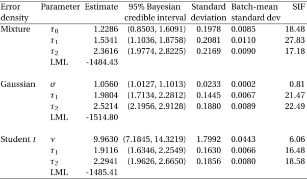
These values are often used as the parameter values of an inverse Gamma density when it is chosen as the prior of a variance parameter (see alsoGeweke,2009). The burn-in period contains 1,000 draws, and the following 10,000 draws were recorded. Whenever the random-walk Metropolis algorithm was used, the acceptance rate was controlled to be between 0.2 and 0.3. The posterior means of the re-parameterized bandwidths are presented in the first panel of Table1. The mixing performance of this posterior sampler is examined by the simulation inefficiency factor (SIF), which can be loosely interpreted as the number of draws needed so as to obtain independent draws from the simulated Markov chain. For example, a SIF value of 20 indicates that approximately, we would need to keep one draw for every 20 draws so as to derive independent draws (see for example,Roberts,1996;Kim, Shephard, and Chib,1998;
Tse, Zhang, and Yu,2004).
The standard deviation of the posterior mean is approximated by the batch-mean standard deviation. It becomes smaller and smaller with the number of simulation iterations increasing, if the sampler achieves a reasonable mixing performance. The SIF and batch-mean standard deviation were used to monitor the mixing performance. Table1presents the values of these two indicators, which show that the sampler has mixed very well.
Under the assumption of Gaussian errors, we usedZhang et al.’s (2009) simulation algo-rithm to sample the re-parameterized bandwidths and the variance parameter from their conditional posteriors, where the re-parameterization was carried out according to (4). The priors of the re-parameterized bandwidths are the same as those under the mixture Gaussian error density. The prior ofσ2is the inverse Gamma density with hyperparametersασ=1 and
βσ=0.05. The results are given in the second panel of Table1.
Assuming the errors of (16) follow the Studenttdistribution withνdegrees of freedom, we derived the likelihood and posterior in a similar way as those derived under Gaussian errors.
The priors of the re-parameterized bandwidths are the same as those under Gaussian errors, and the prior ofνis the Gaussian density with mean 10 and variance 52, which is truncated at 3 with the functional form given by
π(ν)=1/5φ((ν−10)/5)
1−Φ((3−10)/5), (17) whereΦ(·) is the cumulative density function (CDF) of the standard Gaussian distribution. This prior is flat and restrictsνto be greater than 3.
We used the random-walk Metropolis algorithm to sample the re-parameterized band-widths andνfrom their posterior. The results are presented in the third panel of Table1. Under these two parametric assumptions, the values of the SIF and batch-mean standard deviation indicate that both samplers have achieved a reasonable mixing performance.
For each error-density assumption of the nonparametric regression model given by (16), we computed the marginal likelihood given by (14) and the average squared error (ASE) defined as ASE(h)= 1 n n X i=1 [mb(xi,h)−m(xi)]2.
We found the following evidence from this simulation study. First, the marginal likelihood obtained under the mixture Gaussian error density is larger than that obtained under either the Gaussian or Studentterror density. The Bayes factors of the mixture Gaussian error density are exp(20.48) against the Studentt, and exp(32.79) against the Gaussian error densities, respectively. Therefore, the assumption of the mixture Gaussian error density is favored against its parametric counterparts with very strong evidence. Nonetheless, we cannot draw a conclusion only based on one simulated sample. In Section3.3, we calculate the marginal likelihood under each assumption of the error density for 1,000 samples that are independently drawn.
Second, even though the estimated bandwidth vectors in the NW estimator under three assumptions of error density are almost the same, their associated ASEs are different. The ASE derived under the mixture Gaussian error density is 0.0661, which is smaller than that derived under either the Gaussian or Studentterror density.
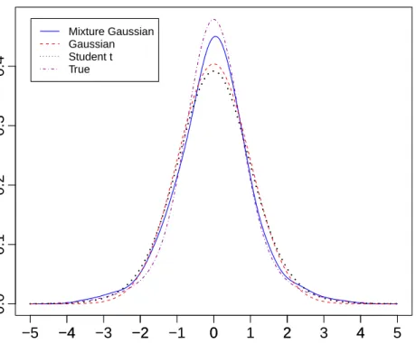
Third, we obtained an estimate of the bandwidth for the kernel error-density estimator, whose graph is plotted in the top panel of Figure1, along with the graphs of the true density, the Gaussian and Studentterror densities. Among these three error-density assumptions, the one derived under the mixture Gaussian error density is the closest to the true density. Moreover, we also plotted the corresponding CDF in the bottom panel of Figure1. As the goodness of fit of the resulting NW estimator is only about 69.4% under each error-density assumption, we believe the error-density estimator obtained under the mixture Gaussian error density performs reasonably well.
3.3 Accuracy of the estimated bandwidth vectors
The accuracy of chosen bandwidths is measured by the ASE of the resulting NW estimator of the true regression function. In kernel density estimation of directly observed data, the NRR is often used for bandwidth selection (see for example,Silverman,1986;Scott,1992;Bowman and Azzalini,1997).Härdle and Müller(2000) indicated that methods for bandwidth selection in nonparametric regression are the same as those for kernel density estimation. Therefore, we considered the NRR for bandwidth selection in the nonparametric regression model in this simulation study.
The likelihood CV for bandwidth selection has been extensively discussed (see for example,
Wahba and Wold,1975;Härdle and Marron,1985;Härdle and Müller,2000). The bootstrapping approach to bandwidth selection in nonparametric regression was presented byHall et al.
(1995), where two pilot bandwidths have to be specified before bootstrapping begins. The purpose of the first bandwidth is to generate a bootstrapping sample, while the second aims to obtain an initial estimate of the regression function. In our simulation study, the two pilot bandwidths were chosen using the NRR and likelihood CV.
For the purpose of generating samples, the error densities we considered are the Gaussian, Studentt and a mixture of two Gaussian densities. We generated 1,000 samples through the regression function given by (15) based on each of the three densities of the errors. For each sample, we chose bandwidths for the NW estimator through the NRR, likelihood CV
and bootstrapping, and derived the estimates of the re-parameterized bandwidths through Bayesian sampling under each of the three assumptions of the error density. As with the Bayesian sampling method, we also estimated the re-parameterized bandwidth for the kernel error-density estimator, as well asσandνunder the Gaussian and Studentt error densities, respectively.
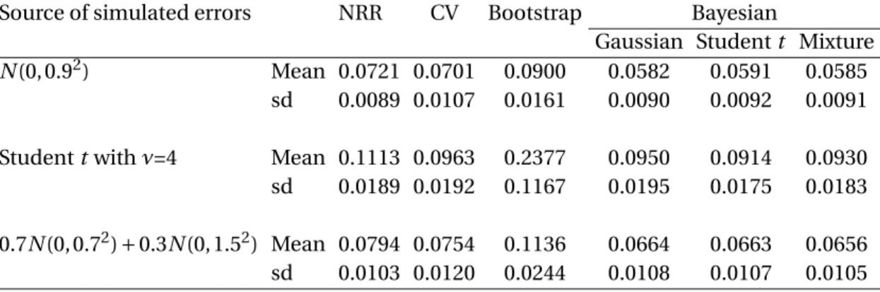
We calculated the ASE of the NW estimator of the regression function with bandwidths estimated through the aforementioned methods. The mean and standard deviation of the 1,000 ASE values were calculated and tabulated in Table2. When the errors were generated fromN(0, 0.92), the mean ASE derived through Bayesian sampling with any error-density as-sumption is smaller than that derived through either the NRR, likelihood CV or bootstrapping. In addition, different assumptions of the error density make no obvious difference in the resulting mean ASE values.
When errors were generated from the Studentt density with 4 degrees of freedom, the mean ASE derived through Bayesian sampling with any error-density assumption is again smaller than that derived through either the NRR, likelihood CV or bootstrapping. The mean ASE obtained through Bayesian sampling under the Gaussian error density is slightly smaller than that obtained through the likelihood CV. Moreover, bootstrapping is clearly the worst performer among all four methods considered.
When the errors were generated from the mixture of two Gaussian densities defined as 0.7N(0, 0.72)+0.3N(0, 1.52), the mean ASE derived through Bayesian sampling under any error-density assumption is clearly smaller than that derived through either the NRR, likelihood CV or bootstrapping. In addition, different assumptions of the error density lead to similar mean ASE values.
3.4 Bayesian comparison among error-density assumptions
The benefit of the mixture Gaussian error density assumption is to gain robustness in terms of error-density specification, because this mixture density is a kernel density estimator of residuals, and has the capacity to approximate an unknown error density. In the
nonpara-metric regression model given by (1), the assumption of a mixture Gaussian error density does not outperform its parametric counterparts under correct error-density assumptions. However, this mixture density usually outperforms its parametric counterparts under wrong assumptions of the error density. We conducted a simulation study using the same 1,000 samples in Section3.3to illustrate this.
3.4.1 Comparison when errors were simulated from Gaussian distribution
For those samples generated by simulating the errors of (15) fromN(0, 0.92), we applied the Bayesian sampling methods to estimate the parameters in (16), where the error density was assumed to be either the Gaussian with mean zero and varianceσ2, the Student t withν degrees of freedom or the mixture Gaussian density given by (8). The Bayesian sampling algorithm under each error-density assumption was applied to each of the 1,000 generated samples. Under each error-density assumption, we derived the estimates of all parameters and marginal likelihood for each sample. We also computed the mean and standard deviation of the 1,000 values of each estimated parameter. Table3presents a summary of these results, where the mean of the SIF values computed under each assumption of the error density is below 16. This finding indicates that the Bayesian sampling algorithms have mixed very well.
As the Gaussian error assumption is correct, we calculated the Bayes factors of the assump-tion of Gaussian error density against the assumpassump-tions of Studentt and mixture Gaussian error densities. According to theJeffreys(1961) scales modified byKass and Raftery(1995), the assumption of Gaussian error density is favored against the Studenttassumption with either strong or very strong evidence in 98.8% of simulated samples. In only 40.6% of simu-lated samples, the Gaussian assumption is favored with either strong or very strong evidence against the mixture Gaussian error density. Moreover, our assumption of a mixture Gaussian error density is favored with either positive, strong or very strong evidence against the correct assumption of the error density in 8.7% of simulated samples. Therefore, on average, the assumption of a mixture Gaussian error density is not favored against the correct assumption of the error density .
3.4.2 Comparison when errors were simulated from Studenttdistribution
We generated samples by simulating the errors from the Studentt distribution withν=4. The Bayesian sampling method was used to estimate all parameters in the nonparametric regression model given by (16), where we considered three assumptions of the error density. We found that the mean of the 1,000 SIF values of each parameter is below 17, which indicates a very reasonable mixing performance of all three samplers. We obtained the mean and standard deviation of the 1,000 values of each estimated parameter under three different assumptions of the error density. We also calculated the marginal likelihood under three assumptions of the error density using each simulated sample. As the Studentterror density is the correct assumption, we calculated the Bayes factors of the Studenttassumption of the error density against the other two assumptions, respectively. A summary of these results is presented in the second panel of Table3.
According to the modified Jeffreys scales, the assumption of Studentterrors is favored with either strong or very strong evidence against the Gaussian assumption in all simulated samples, and against the assumption of mixture Gaussian errors in 90.1% of simulated sam-ples. However, the mixture Gaussian error-density assumption is favored with either positive, strong or very strong evidence against the correct assumption in 2.7% of simulated samples. This finding shows that on average, the assumption of mixture Gaussian error density is not favored against the correct assumption of the error density.
3.4.3 Comparison when errors were simulated from mixture Gaussian distribution We simulated samples by drawing errors from a mixture of two Gaussian distributions defined as 0.7N(0, 0.72)+0.3N(0, 1.52). The Bayesian sampling method under each of the three error-density assumptions, was applied to estimate parameters in the nonparametric regression model. According to Bayes factors, we derived the estimates of parameters and marginal likelihood for each sample under three assumptions of the error density. We made decisions on whether the assumption of the mixture Gaussian error density is favored against the other two assumptions for each simulated sample. A summary of these results is given in the third
panel of Table3.
All three assumptions of the error density led to similar estimates of the bandwidth vector in the NW estimator. The mean of SIF values for each parameter under three assumptions of the error density is below 16. This indicates a very good mixing performance of all three samplers.
As the errors were generated from a mixture of two Gaussian densities, all three assump-tions of the error density are inaccurate. The assumption of Gaussian errors is likely to lead to poorer performance than the other two, because the true error density exhibits heavy tails. According to the computed Bayes factors and the modified Jeffreys scales, the mixture Gaussian assumption of the error density is favored against the Gaussian assumption in 99.2% of simulated samples, and against the Studentt assumption in 60.7% of simulated samples. In comparison, the Studenttassumption is favored against the mixture Gaussian assumption in only 27.0% of simulated samples. Moreover, we found that the assumption of the mixture Gaussian error density is favored with either strong or very strong evidence against the assumption of the Studentterror density in 49.2% of simulated samples. On the other hand, the latter assumption is favored against the former with the same strength of evidence in only 16.3% of simulated samples. Thus, we can conclude that when the error density is unknown, our proposed mixture Gaussian error density is often favored against its parametric counterparts with wrong error-density assumptions.
3.5 Sensitivity of prior choices
Current asymptotic results show that as the sample size tends to infinity, the two types of bandwidths approach zero asymptotically. When there are three or more regressors in the nonparametric regression model,Samb(2010) proved that the optimal rates aren−3/(2d+11)for the bandwidth in the kernel density estimator of residuals andn−1/(d+4)for the bandwidths
Therefore, we assume that the prior densities ofbandhi are the uniform densities given by b∼U¡ 0, 2σεn−3/17+1/10¢ , (18) hk∼U ¡ 0, 2σkn−1/7+1/10 ¢ , (19)
whereσεis the standard deviation of residuals, andσk is the standard deviation of thekth
regressor, fork=1, 2, . . . ,d. The optimal rates were scaled up byn1/10to guarantee that the most appropriate values of bandwidths are within the intervals.
Replacing the prior densities in (13) with the uniform priors defined by (18) and (19), we derived the approximate posterior ofhandb, through which we sampled the parameters using the random-walk Metropolis algorithm for each of the 1,000 samples in Section3.2. Moreover, we used the uniform priors given by (19) to derive the approximate posterior for the nonparametric regression model with either the Gaussian or Studentterrors. We derived the estimate of the parameter vector by implementing the same posterior sampler for each sample. A summary of the simulation results is presented in Table4.
Transforming the estimatedτvalues reported in Table3into bandwidth values according to (4), we found that over the 1,000 generated samples, the means of the posterior estimates of the parameter vector obtained under the uniform priors are similar to those obtained under the inverse Gamma priors for each assumption of the error density. Therefore, the posterior estimate of the parameter vector obtained through the aforementioned posterior samplers is on average, insensitive to different prior choices of the bandwidth parameters. Nonetheless, the decisions on whether one assumption of the error density is favored against the others under the uniform priors are different from those under the inverse Gamma priors.
When the errors were generated from the Gaussian distribution, the assumption of Gaus-sian errors is favored against the assumption of Studentterrors with either strong or very strong evidence in 99.7% of simulated samples under the uniform priors. This relative fre-quency is similar to the relative frefre-quency of 98.8% under the inverse Gamma priors. On the other hand, the Gaussian assumption is favored against the mixture Gaussian error density with either strong or very strong evidence in 48.3% of simulated samples under the uniform priors, rather than 40.6% of simulated samples under the inverse Gamma priors.
When the errors were generated from the Studenttdistribution, the decisions on whether the Studenttassumption is favored against the other two under the uniform priors are largely the same as those under the inverse Gamma priors.
When the errors were generated from the mixture of two Gaussian densities, the pro-posed mixture Gaussian error density is favored with either positive, strong or very strong evidence against the Gaussian and Studentt error densities in respectively, 99.6% and 73.7% of the simulated samples, under the uniform priors. The latter value is clearly larger than its counterpart, which is 60.7%, under the inverse Gamma priors.
To summarize, on average, the estimated bandwidths are largely insensitive to prior choices. Nonetheless, when samples were generated from either the Gaussian or the mixture Gaussian error distributions, the assumption of a mixture Gaussian error density is more frequently favored against the Studenttassumption under uniform priors than under inverse Gamma priors.
4 An application to nonparametric regression of stock returns
To investigate the empirical relevance of the Bayesian bandwidth selectors, we applied them to the nonparametric regression of the All Ordinaries daily return on the overnight returns of FTSE and S&P 500. As the opening time for share trading in the Australian stock market is after the closing time of the previous-day trading in the UK and USA stock markets, such an investigation can reveal the relationship between the Australian stock market and the other two markets.4.1 Data
The data consist of the All Ordinaries, FTSE and S&P 500 closing indices collected from the 3rd January 2007 to the 30th March 2011, excluding non-trading days. The All Ordinaries daily return was matched to the overnight FTSE and S&P 500 returns. As a consequence, the daily returns of the FTSE and S&P 500 indices on the 30th March 2011 (local time) was not used for the purpose of estimating bandwidths. When one market experienced a
non-trading day, we also deleted the non-trading data in the other two markets on that day. The sample containsn=1, 022 observations, from which we computed continuously compounded daily percentage returns. We employ the multivariate nonparametric regression model given by
yi=m(x1,i,x2,i)+εi, fori=1, 2, . . . ,n, (20)
whereyi is the return of the All Ordinaries daily index, andε1,ε2, . . . ,εnare assumed to be iid
with their distributions assumed to be Gaussian, Studenttand mixture Gaussian, respectively.
4.2 Bandwidth estimates under different error densities
As Bayesian sampling was used to estimate the re-parameterized bandwidths (and the pa-rameter under each parametric assumption of the error density), we re-papa-rameterized the bandwidths for the NW estimator of the regression function ashk=τkn−1/6, fork=1 and 2,
under each of the three assumptions of the error density. The prior ofτ2kgiven by (12), was chosen by assuming thatτ2kn−2/6follows IG(αh,βh) withαh=1 andβh=0.05, under each assumption of the error density.
When the error density of (20) are assumed Gaussian with mean zero and varianceσ2, we chose the prior ofσ2as IG(1,0.05). Note that our prior choices forσ2andτ2k, fork=1 and 2, are different from those inZhang et al.(2009). The random-walk Metropolis algorithm was used to sampleτ21andτ22from their conditional posterior, while the Gibbs sampler was used to sampleσ2from its conditional posterior. We used the batch-mean standard deviation and SIF to examine the mixing performance of the sampling algorithm. Both the batch-mean standard deviation and SIF indicate that all simulated chains have achieved a reasonable mixing performance with the SIF values below 35. Table5presents the estimates ofσand the elements ofτ, and their associated statistics. During the MCMC iterations, we obtained the 95% Bayesian credible interval of each element of the bandwidth vector, which cannot be obtained through the NRR, likelihood CV and bootstrapping.
When the errors are assumed to follow the Studenttdistribution withνdegrees of freedom, we assumed that the prior ofνis a truncated Gaussian density given by (17) and used the random-walk Metropolis algorithm to sampleνand the elements ofτ2. Table5presents
the estimated (ν,τ1,τ2)0, and its associated statistics. According to the batch-mean standard deviation and SIF, each simulated chain has mixed well. As the estimate ofνis small, this indicates a slightly heavy-tailed behavior of the error density. As a consequence, it leads to a different distributional shape in comparison with the Gaussian error density.
When the errors are assumed to follow the mixture of Gaussian densities given by (8), the bandwidth for the kernel-form error density was re-parameterized asb=τ0n−1/5. The prior ofτ20given by (11), was chosen by assuming thatτ20n−2/5follows IG(αb,βb) withαb=1 and
βb=0.05. We used the random-walk Metropolis algorithm to sampleτ2k, fork=0, 1 and 2,
from their posterior given by (13). Table5presents the estimatedτk, fork=0, 1 and 2, and
their associated statistics. According to the batch-mean standard deviation and SIF values, all simulated chains have achieved a reasonable mixing performance.
4.3 Comparison of different error-density assumptions
We computed the Bayes factors with marginal likelihoods calculated through (14), where the marginal likelihood derived under each assumption of the error density is shown in Table5. The marginal likelihood under the mixture Gaussian error density is found to be slightly larger than that under the Studentt errors, while the Bayes factor reveals no sufficient evidence to make a decision on whether the former assumption is favored against the latter due to narrow difference between the two marginal likelihood values. However, the assumption of the mixture Gaussian error density is favored against the assumption of Gaussian error density with very strong evidence.
Conditional on the overnight daily returns of the FTSE and S&P 500 indices on the 30th March 2011 (local time), we forecasted the daily return of the All Ordinaries index on the 31st March 2011 (local time) before the Australian stock market opened. Under each assumption of the error density, we derived the posterior estimates of the re-parameterized bandwidths for the NW estimator of the regression function, which was computed at the daily returns of FTSE and S&P 500 on the 30th March 2011 to derive a point forecast of the daily return of the All Ordinaries index on the 31st March 2011. We also produced such a point forecast
at each iteration of the MCMC simulation so as to obtain a posterior sample of the point forecast, based on which we derived the 95% Bayesian credible interval for the point forecast on the All Ordinaries index on the 31st March 2011. Under the three assumptions of the error density, the point forecasts are respectively, 0.2663%, 0.2562% and 0.2676%; and the corresponding credible intervals are respectively, (0.2449%, 0.2885%), (0.2381%, 0.2736%) and (0.2486%, 0.2905%).
4.4 Error-density estimators under different assumptions
Under the Gaussian-component mixture density of the errors, we are able to estimate the density of the one-step-ahead point forecast of the All Ordinaries daily return, and the derived density can be regarded as a density forecast. Using the estimated bandwidths and parameters given in Table5, we derived the density of the point forecast of the All Ordinaries daily return on the 31st March 2011 under each of the three assumptions of the error density. The graphs of the three derived densities are presented in Figure2. The three density graphs are obviously different to each other at their peaks and left tails. As the sample period covers the current global financial crisis, the heavy-tailed feature of stock index-return during this period is more evident than that during non-crisis periods. Consequently, the heavy-tailed mixture Gaussian and Studenttdensities are favored against the Gaussian according to Bayes factors. During the period of global financial crisis, global stock markets had experienced very frequent huge drops. Therefore, the estimated density of the point forecast of the All Ordinaries return obtained through the Gaussian-component mixture density of errors exhibits a thick left tail. This distributional feature cannot be revealed through the assumption of Studentterrors.
Under each of the three estimated densities of the All Ordinaries daily return, we computed the one-day VaR for holding an investment on the All Ordinaries index on the 31st March 2011. At the 95% confidence level, the one-day VaRs are respectively, $1.5668, $1.5452 and $1.4803 for every $100 investment on the All Ordinaries index under the assumptions of the mixture Gaussian, Studenttand Gaussian error densities. In light of the fact that many financial firms had experienced severe liquidity stress or even filed for bankruptcy during the global financial
crisis, we tend to believe that market risk had been underestimated. Therefore, we believe that in comparison to the mixture Gaussian error density, the assumption of Gaussian errors leads to an underestimated VaR.
5 An application to SPD estimation
Aït-Sahalia and Lo(1998) showed that in a dynamic equilibrium model, the price of a security is Pt=exp © rt,λλ ª Et∗{Z(ST)}=exp © rt,λλ ª Z ∞ −∞ Z(ST)ft∗(ST)d ST,
whereT =t+λ,λis the length of time to maturity,rt,λis a constant risk-free interest rate
betweentandT,E∗t represents the expectation taken conditional on information available at
datet,ST is the price of the security at dateT,Z(ST) is the payoff of the security at the expiry
dateT, andft∗(ST) is the date-tSPD for the payoff of the security at dateT. When an option is
the security of interest, the SPD is the second-order derivative of a call-option pricing formula with respect to strike price calculated atST.Aït-Sahalia and Lo(1998) showed that the date-t
price of a call option, is a nonlinear function of (St,Xt,λ,rt,λ,δt,λ)0, which can be estimated through the nonparametric regression technique, whereδt,λis the dividend rate at datet.
In order to reduce the number of regressors,Aït-Sahalia and Lo(1998) assumed that the call-option pricing formula is given by the Black-Scholes (BS) formula except that the date-t volatility denoted byσt, is estimated by the nonparametric regression of the implied volatility
onzet =(Ft,X,δ), whereFt is the futures price of the underlying asset. The kernel estimator of
the regression function is
b σt(Ft,X,λ|h)= n−1Pn j=1Kh(zet−z˜j)σej n−1Pn j=1Kh(zet−zej) ,
whereσejis the volatility implied by the price of the call option, andhis a vector of bandwidths.
the risk measures of delta (∆) and Gamma (Γ) are expressed as fB S,t(ST)= 1 ST p 2πσ2λexp ½ −[ln(ST/St)−(rt,λ−δt,λ−σ 2/2)λ]2 2σ2λ ¾ , ∆B S=Φ(d1), ΓB S= φ(d1) Stσ p λ. whered1= © ln(St/X)+(rt,λ−δt,λ+σ2/2)λ ª /(σλ1/2).
Zhang et al.(2009) assumed that the errors of the nonparametric regression model of
e
σt onezt follow the Gaussian distribution with a zero mean and unknown variance. In this
paper, we assume that the errors of this nonparametric regression model follow the mixture of Gaussian densities given by (2). We fitted the model to the S&P 500 index options data, which are the same as those investigated byAït-Sahalia and Lo(1998) andZhang et al.(2009). The sample period is from the 4th January to the 31st December 1993, and the sample size isn=14, 431. We applied the sampling procedure proposed in Section2.2 to sample the re-parameterized bandwidths from their posterior. Table6presents the estimates of the re-parameterized bandwidths and some associated statistics. Transforming the estimated
τvalues into bandwidths according to (4), we found that the bandwidth vector for the NW estimator is (4.9810, 4.7884, 13.8418)0. This is clearly different from (5.6243, 5.4831, 9.7509)0
derived under the assumption of Gaussian error density. The bandwidth for the kernel-form error density is 0.2424.
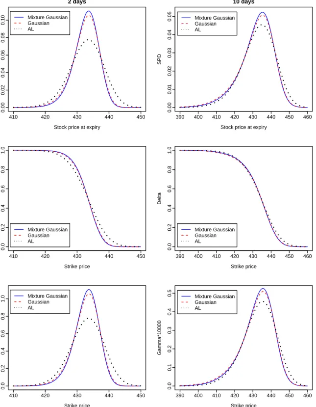
The Bayes factor of the mixture Gaussian error density against the Gaussian error density is exp(4210.13), which is very strong evidence supporting the former. Using the bandwidth vector derived byAït-Sahalia and Lo(1998), and the ones estimated through Bayesian sam-pling under both error densities, we plotted the graphs of the SPD, the risk measures∆andΓ at maturities of 2 and 10 days, respectively, in Figure3. At the maturity of 2 days, the SPD and Γproduced through the bandwidth vector derived under the mixture Gaussian error density are respectively, different from those derived under the Gaussian error density. However, as the time to maturity increases to 10 days, both densities lead to similar estimates of the SPD andΓ.
Moreover, the SPD,∆andΓderived through Bayesian sampling under each assumption of the error density are clearly different from those derived through the rule-of-thumb reported byAït-Sahalia and Lo(1998). However, different assumptions of the error density lead to similar estimates of the SPD, risk measures∆andΓwhen maturity is 25 days or more.
6 Conclusion
We have presented a Bayesian approach to the estimation of bandwidths for the Nadaraya-Watson regression estimator and kernel-form error density estimator in the nonparametric regression model. The unknown error density is approximated by the mixture of Gaussian densities centered at individual error realizations and scaled by a constant parameter or the bandwidth in the context of kernel smoothing. We have conducted a series of simulation studies, which reveal that our approach outperforms the normal reference rule, likelihood cross-validation and bootstrapping methods in estimating the bandwidths for the Nadaraya-Watson estimator (as measured by ASE). In comparison to the parametric assumption of either the Gaussian or Studentterror density, our proposed mixture Gaussian error density or equivalently the kernel-form density estimator of residuals, is not favored against the correct error-density assumption, but is favored against wrong assumptions of the error density. Our Bayesian sampling procedure represents a data-driven solution to the problem of simultaneously estimating bandwidths for the kernel estimators of the regression function and error density.
Applying to the nonparametric regression of the All Ordinaries daily return on the overnight FTSE and S&P 500 returns, we have obtained the bandwidth estimates for the kernel estimator of the regression under the three error-density assumptions. Although the assumption of a Gaussian-component mixture error density performs on par with the assumption of the Studentterror density, they both outperform the Gaussian error-density assumption. The density estimator of the All Ordinaries daily return obtained through the mixture Gaussian error density exhibits a more reasonable left-tail behavior than that obtained through either the Gaussian or Studentterror density. Moreover, under the Gaussian-component mixture
error density, we are able to estimate the density of the one-step-ahead point forecast of the All Ordinaries return. Therefore, the resulting value-at-risk is distribution-free and gain robustness in terms of different specifications of the error density.
We have also employed the proposed Bayesian sampling algorithm to estimate bandwidths for the nonparametric regression model involved in the state-price density estimation, where the error density is approximated by the Gaussian-component mixture density of the errors. The assumption of such an error density is favored with very strong evidence against the assumption of Gaussian error density. Moreover, we have found that the state-price density, risk measures∆and Γ estimated under this mixture error density are different from the corresponding ones estimated under Gaussian assumption errors at short maturities of the underlying asset. This example confirms the usefulness of relaxing the Gaussian assumption of the error density to a kernel-form or equivalently the Gaussian-component mixture error density in a nonparametric regression model.
Acknowledgements
We extend our sincere thanks to John Geweke and Peter Robinson for their very insightful comments on an earlier draft of this paper. Thanks also go to the Victorian Partnership for Advanced Computing (VPAC) for its quality computing facility. This research was supported under the Australian Research Council’sDiscovery Projectsfunding scheme (project number DP1095838).
References
Aït-Sahalia, Y., Lo, A. W., 1998. Nonparametric estimation of state-price densities implicit in financial asset prices. The Journal of Finance 53 (2), 499–547.
Bowman, A. W., Azzalini, A., 1997. Applied Smoothing Techniques for Data Analysis. Oxford University Press, London.
Brewer, M. J., 2000. A Bayesian model for local smoothing in kernel density estimation. Statis-tics and Computing 10 (4), 299–309.
Cheng, F., 2004. Weak and strong uniform consistency of a kernel error density estimator in nonparametric regression. Journal of Statistical Planning and Inference 119 (1), 95–107. Chib, S., 1995. Marginal likelihood from the Gibbs output. Journal of the American Statistical
Association 90 (432), 1313–1321.
de Lima, M. S., Atuncar, G. S., 2011. A Bayesian method to estimate the optimal bandwidth for multivariate kernel estimator. Journal of Nonparametric Statistics 23 (1), 137–148.
Efromovich, S., 2005. Estimation of the density of regression errors. The Annals of Statistics 33 (5), 2194–2227.
Gangopadhyay, A., Cheung, K., 2002. Bayesian approach to the choice of smoothing parameter in kernel density estimation. Journal of Nonparametric Statistics 14 (6), 655–664.
Gelfand, A. E., Dey, D. K., 1994. Bayesian model choice: Asymptotics and exact calculations. Journal of the Royal Statistical Society, Series B 56 (3), 501–514.
Geweke, J., 2009. Complete and Incomplete Econometric Models. Princeton University Press, New Jersey.
Geweke, J. F., 1999. Using simulation methods for Bayesian econometric models: Inference, development, and communication. Econometric Reviews 18 (1), 1–73.
Hall, P., Lahiri, S. N., Polzehl, J., 1995. On bandwidth choice in nonparametric regression with both short-and long-range dependent errors. The Annals of Statistics 23 (6), 1921–1936. Härdle, W., 1990. Applied Nonparametric Regression. Cambridge University Press, Cambridge. Härdle, W., Hall, P., Ichimura, H., 1993. Optimal smoothing in single-index models. The Annals
of Statistics 21 (1), 157–178.
Härdle, W., Marron, J. S., 1985. Optimal bandwidth selection in nonparametric regression function estimation. The Annals of Statistics 13 (4), 1465–1481.
Härdle, W., Müller, M., 2000. Multivariate and semiparametric kernel regression. In: Schimek, M. G. (Ed.), Smoothing and Regression: Approaches, Computation, and Application. John Wiley & Sons, New York, pp. 357–392.
Herrmann, E., Engel, J., Wand, M. P., Gasser, T., 1995. A bandwidth selector for bivariate kernel regression. Journal of the Royal Statistical Society, Series B 57 (1), 171–180.
Huynh, K., Kervella, P., Zheng, J., 2002. Estimating state price densities with nonparametric re-gression. In: Härdle, W., Kleinow, T., Stahl, T. (Eds.), Applied Quantitative Finance. Springer Verlap, Heidelberg.
Jeffreys, H., 1961. Theory of Probability. Oxford University Press, Oxford, U.K.
Kass, R. E., Raftery, A. E., 1995. Bayes factors. Journal of the American Statistical Association 90 (430), 773–795.
Kim, S., Shephard, N., Chib, S., 1998. Stochastic volatility: Likelihood inference and compari-son with ARCH models. Review of Economic Studies 65 (3), 361–393.
Linton, O., Xiao, Z., 2007. A nonparametric regression estimator that adapts to error distribu-tion of unknown form. Econometric Theory 23 (3), 371–413.
Muhsal, B., Neumeyer, N., 2010. A note on residual-based empirical likelihood kernel density estimation. Electronic Journal of Statistics 4, 1386–1401.
Newton, M. A., Raftery, A. E., 1994. Approximate Bayesian inference with the weighted likeli-hood bootstrap. Journal of the Royal Statistical Society, Series B 56 (1), 3–48.
Roberts, G. O., 1996. Markov chain concepts related to sampling algorithms. In: Gilks, W. R., Richardson, S., Spiegelhalter, D. J. (Eds.), Markov Chain Monte Carlo in Practice. Chapman & Hall, London, pp. 45–57.
Rothe, C., 2009. Semiparametric estimation of binary response models with endogenous regressors. Journal of Econometrics 153 (1), 51–64.
Samb, R., 2010. Nonparametric kernel estimation of the probability density function of re-gression errors using estimated residuals. working paper, Universite Pierre et Marie Curie, LSTA.
URLhttp://arxiv4.library.cornell.edu/abs/1010.0439
Scott, D. W., 1992. Multivariate Density Estimation: Theory, Practice, and Visualization. Wiley, New York.
Silverman, B. W., 1978. Weak and strong uniform consistency of the kernel estimate of a density and its derivatives. The Annals of Statistics 6 (1), 177–184.
Silverman, B. W., 1986. Density Estimation for Statistics and Data Analysis. Chapman and Hall, New York.
Tse, Y. K., Zhang, X., Yu, J., 2004. Estimation of hyperbolic diffusion using the Markov chain Monte Carlo method. Quantitative Finance 4 (2), 158–169.
Wahba, G., Wold, S., 1975. A completely automatic French curve: Fitting spline functions by cross validation. Communications in Statistics — Theory and Methods 4 (1), 1–17.
Wand, M. P., Jones, M. C., 1995. Kernel Smoothing. Chapman and Hall, New York.
Yuan, A., de Gooijer, J. G., 2007. Semiparametric regression with kernel error model. Scandi-navian Journal of Statistics 34 (4), 841–869.
Zhang, X., Brooks, R. D., King, M. L., 2009. A Bayesian approach to bandwidth selection for multivariate kernel regression with an application to state-price density estimation. Journal of Econometrics 153 (1), 21–32.
Zhang, X., King, M. L., 2010. Bayesian semiparametric GARCH models.Bayes on the Beach, 4–5 October, Gold Coast, Australia.