Optimal power flow solution with uncertain RES using augmented grey wolf optimization

(1)

Optimal Power Flow Solution with Uncertain RES

using Augmented Grey Wolf Optimzation

Inam Ullah Khan

1,∗

, Nadeem Javaid

2

, C. James Taylor

1

, Kelum A. A Gamage

3

and Xiandong MA

1

1_{Engineering Department, Lancaster University, Bailrigg, Lancaster LA1 4YW, UK} 2_{Department of Computer Science, COMSATS University Islamabad, Islamabad, 44000, Pakistan}

3_{James Watt School of Engineering, University of Glasgow, Glasgow G12 8QQ, UK}

*Correspondence: [email protected]

Abstract—This work focuses on implementing the optimal power flow (OPF) problem, considering wind, solar and hy-dropower generation in the system. The stochastic nature of renewable energy sources (RES) is modelled using Weibull, Log-normal and Gumbel probability density functions. The system-wide economic aspect is examined with additional cost functions such as penalty and reserve costs for under and overestimating the imbalance of RES power outputs. Also, a carbon tax is imposed on carbon emissions as a separate objective function to enhance the contribution of green energy. For solving the optimization problem, a simple and efficient augmentation to the basic grey wolf optimization (GWO) algorithm is proposed, in order to enhance the algorithm’s exploration capabilities. The performance of the new augmented GWO (AGWO) approach, in terms of robustness and scalability, is confirmed on IEEE-30, 57 and 118 bus systems. The obtained results of the AGWO algorithm are compared with modern heuristic techniques for a case of OPF incorporating RES. Numerical simulations indicate that the proposed method has better exploration and exploitation capabilities to reduce operational costs and carbon emissions.

Index Terms—Optimal power flow, Renewable energy sources, Carbon emission, Meta-heuristic techniques

I. INTRODUCTION

Optimal power flow (OPF) has proved to be an essential tool for the efficient and secure operation of power networks since its inception. The main objective of OPF is to find optimal set-tings of the control variables with certain objective functions while satisfying system equality and inequality constraints. The system control variables that need adjustment include generated active power, the voltage of all generation buses and tap settings of the transformer. During the optimization process, system constraints such as transmission line capacity, power flow balance, voltage profile of all buses and generator capability constraints need to be maintained.

OPF with only traditional thermal power generators (TPGs) is widely studied in the literature [1]. However, with increased penetration of RES, it is necessary to incorporate associated uncertainty into the power network. Under recent studies, sys-tems that consider both TPGs and RES are in pursuit of similar objective functions studied in the past [2]–[6]. The work in [2] conducts an extensive study on the over/underestimation of wind power generation (WPG) in the classical economic dispatch model. In this study, the Weibull probability density function (PDF) is used to model the uncertainty of WPG output. For economic dispatch strategies, it provides valuable

insight into the integrated wind system. However, the chal-lenge of wind speed variation on the optimal dispatch schedule of power plants remains unaddressed. Also, the reactive power capability of WPGs, bus voltage constraints and loading effect of transmission line were not considered in [3].

Authors in [4] combined advanced variant of differential evolution with an effective constraint handling technique for a system that considers both solar and wind power generation in the OPF problem. The uncertain and intermittent nature of both RES were modelled with lognormal and Weibull PDFs. However, the resulting SHADE-SF algorithm sometimes at-tains premature convergence (i.e., becomes trapped in a local solution) and the convergence rate can be prolonged. The scalability and robustness of the proposed algorithm were not verified since the algorithm was only verified on the IEEE-30 bus system. This does not guarantee good performance over medium and higher bus systems (57 and IEEE-118). In general, OPF with the incorporation of RES needs further attention.

II. MATHEMATICAL MODEL

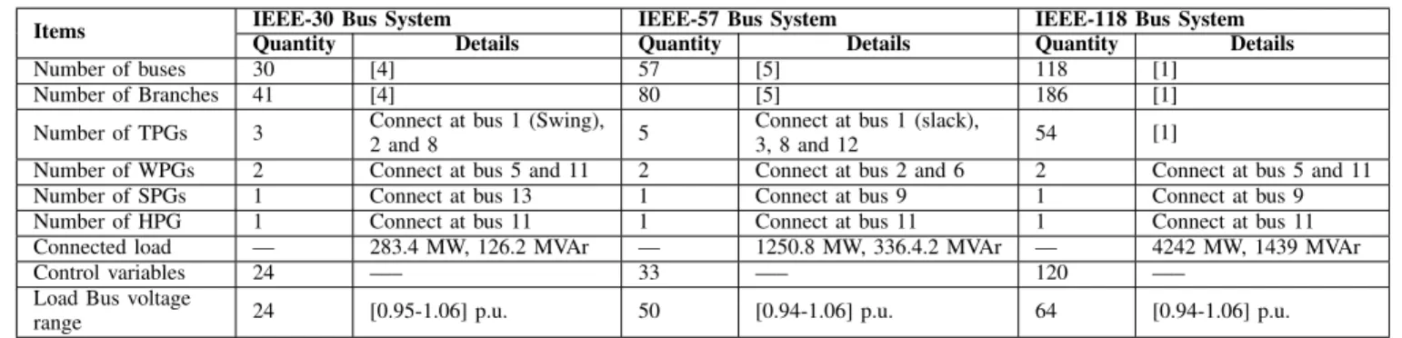
In this work, the IEEE-30, 57 and 118 bus systems are used to validate the performance of the proposed AGWO algorithm in the OPF problem. The essential characteristics of these bus systems are provided in Table I. Along with the TPGs, RES such as wind, solar and small hydro (WSH) generators are selected as power generation sources for the OPF framework. The power output from RES is variable in nature and power output instability needs to be minimized and balanced by the aggregation of the power outputs of all the generators and spinning reserve. Thus, total power generation cost is the combination of operating cost of all generators, reserve and penalty cost (due to the intermittent nature of power generation from RES). In subsequent subsections, cost models are discussed in detail.

A. Stochastic Wind Power

The behaviour of the wind speed v(m/s) distribution can be modelled with the help of Weibull PDFfv(v)by adjusting

scale parameter c and shape parameter k as established by [3] and [4]. The probability of wind speed during any time interval is expressed as follows:

(2)

In the modified IEEE-30 bus system, TPGs at bus 5 and bus 11 are replaced with the WPGs. The values for scalecand shape

k parameters are given in Table II. The wind speed behavior for WPG 1 and WPG 2 at buses 5 and 11 follow the Weibull PDF. For each WPG, the relationship between wind speed and output power is expressed in Eq. 2 [3]:

PW =    0, v < vcior v > vco PW r, vr< v≤vco PW r(_vv−vci r−vci), vci≤v≤vr, (2)

wherev is forecasted wind speed inm/s,vci,vco andvr are

cut-in, cut-out and rated wind speeds, PW r is rated output

power for the WPG.

B. Stochastic Solar Power

Similarly, the TPG at bus 13 of the modified IEEE-30 bus system is replaced with the solar power generator (SPG). The output power from SPG depends upon the solar irradiance which follows lognormal PDF. The probability with standard deviation λand meanσ can be calculated as follows [4]:

fX(X) = 1 Xσ√2πexp ₋_[ln_X₋_λ_]2 2σ2 , X >0 (3) The values forλandσare given in Table II. The relationship between the solar irradiance X (W/m2₎_{and output power of}

SPG is expressed as follows: PS(X) =    PSr( X 2 XstdCI), 0< X < CI PSr(_XX std), X > CI, (4)

whereX is forecasted solar irradiance,Xstd is standard solar

irradiance value set as 800 W/m2_, _C

I is certain irradiance

point (120W/m2_{) and}_P

SR is rated SPG power output. C. Stochastic Hydropower

It is well known that the Gumbel distribution is followed for river flow rate calculations. The probability calculation of Gumbel distribution for river flow rate with scale parameterω

and location parameter γis formulated in Eq. 5 [5]:

fH(Gh) = 1 ωexp −(Gh−γ) ω ) exp −exp(Gh−γ) ω (5) In the modified IEEE 30-bus system, the conventional TPG at bus 13 is replaced together with 45 MW SPG and 5 MW small HPG. Table II provides PDF values for these fittings and many of these values are realistically chosen in a study given by Ref. [5]. The output of HPG as a function of pressure head and water flow rate is calculated as follows:

Ph(Gh) =αβgGhPh (6)

whereαandβ represent efficiency of the generating unit and density of water volume, respectively. The numerical values for calculation of HPG output are assumed:α= 0.85,β 1000 kg/m3_,_P

h = 25m andg = 9.81m/s2.

D. Cost Model for Thermal Power Generators

TPGs require fossil fuel for their operation. The relationship between generated power (MW) and fuel cost ($/h) can be calculated with the help of following quadratic equation:

CT = NT

X

i=1

ai+biPT g,i+ciPT g,i2 (7)

Practically, the valve point loading effect needs to be con-sidered to model accurate cost function. Hence, the overall thermal power generation cost ($/h) becomes:

CT = NT X i=1 ai+biPT g,i+ciPT g,i2 + di×sin ei×(PT g,im −PT g,i) (8) where ai, bi, ci are the cost coefficients and di, ei are fuel

cost coefficients for the i-th TPG. PT g,i is the output power, NT is total number of the TPGs in the system andPT g,im the

minimum power when i-th TPG is in operation. All emission and cost coefficients pertaining to TPGs are given in Table III.

E. Cost Model for Renewable Energy Sources

The total cost of the RES consists of the direct cost associ-ated with scheduled power, reserve cost for overestimation and penalty cost for underestimation. These models are developed in line with the concept presented in Refs. [3]–[6].

The direct, reserve and penalty costs of WPG as a function of scheduled power are represented in Eqs. 9–11 as follows:

CDW,j=dw,jPW S,j (9) CRW,j=rw,j Z PW S,j 0 (PW S,j−W)fw(W)dW (10) CP W,j=pw,j Z PW R,j PW S,j (W−PW S,j)fw(W)dW (11)

wheredw,j,rw,j andpw,j are direct, reserve and penalty cost

coefficients pertaining to j-th WPG. PW S,j is the scheduled

power andfw(W)is PDF of same WPG.

The total cost of WPG can be calculates as:

CT W,j=CDW,j+CRW,j +CP W,j (12)

Likewise, the SPG also has uncertain power output. The direct, reserve and penalty costs pertaining to the k-th SPG are represented as: CDS,k=ds,kPSS,k (13) CRS,k=rs,k·P r(PAS,k< PSS,k)· [(PSS,k−E(PAS,k< PSS,k)] (14) CP S,k=ps,k·P r(PAS,k> PSS,k)· [(E(PAS,k> PSS,k)−PSS,k] (15)

In Eqs. 13–15, ds,k, rs,k and ps,k are direct, reserve and

(3)

TABLE I:Characteristics of Bus Systems under Consideration

Items IEEE-30 Bus System IEEE-57 Bus System IEEE-118 Bus System

Quantity Details Quantity Details Quantity Details

Number of buses 30 [4] 57 [5] 118 [1]

Number of Branches 41 [4] 80 [5] 186 [1]

Number of TPGs 3 Connect at bus 1 (Swing),_{2 and 8} 5 Connect at bus 1 (slack),_{3, 8 and 12} 54 [1]

Number of WPGs 2 Connect at bus 5 and 11 2 Connect at bus 2 and 6 2 Connect at bus 5 and 11

Number of SPGs 1 Connect at bus 13 1 Connect at bus 9 1 Connect at bus 9

Number of HPG 1 Connect at bus 11 1 Connect at bus 11 1 Connect at bus 11

Connected load — 283.4 MW, 126.2 MVAr — 1250.8 MW, 336.4.2 MVAr — 4242 MW, 1439 MVAr

Control variables 24 —– 33 —– 120 —–

Load Bus voltage

range 24 [0.95-1.06] p.u. 50 [0.94-1.06] p.u. 64 [0.94-1.06] p.u.

TABLE II:PDF Parameters for Wind, Solar and Hydropower Generation [4], [5].

Wind power generation plants Solar + Hydropower generation plant (bus 13)

Windfarm # No. of wind turbines Total rated power Weibull PDF parameters Rated power of SPG Lognormal PDF parameters Rated power of HPG Gumbel PDF parameters 1 at bus 5 25 75 MW c = 9, k = 2 45 MW λ= 6,σ= 0.6 5 MW ω= 15,γ= 1.2 2 at bus 11 20 60 MW c = 10, k = 2

TABLE III:Thermal Power Generators Cost and Emission Coefficients for the System [4].

Thermal generator Bus number a b c d e f g h k l

TPG1 1 0 2 0.00375 18 0.037 4.091 -5.554 6.49 0.0002 6.667

TPG2 2 0 1.75 0.0175 16 0.038 2.543 -6.047 5.638 0.0005 3.333

TPG3 8 0 3.25 0.00834 12 0.045 5.326 -3.55 3.38 0.002 2

PSS,k represent available and scheduled power from SPG.

Finally, the total cost of SPG can be calculated as:

CT S,k=CDS,k+CRS,k+CP S,k (16)

As a third RES, we consider a small hydropower generator (HPG) in this study. The output of HPG is very less (10–20 % of total install capacity) [5]. It is therefore combined with SPG and assumed to be owned by a single private operator. Following Eqs 13–15, the direct, reserve cost for overestima-tion and penalty cost for underestimaoverestima-tion of combined solar hydropower generation system is:

CSH =dsPSSH,s+dhPSSH,h (17)

CRSH =rsh,m·P r(PASH< PSSH)·

[(PSSH−E(PASH < PSSH)] (18)

CP SH =psh,m·P r(PASH> PSSH)·

[(E(PASH > PSSH)−PSSH] (19)

where PSSH,s and PSSH,h represent scheduled power from

SPG and HPG, respectively.dh,m,rsh,mandpsh,mare direct,

reserve and penalty cost coefficients pertaining to m-th HPG.

PASH and PSSH represent available and scheduled output

power from combined solar hydropower generator. Finally, the total cost of HPG is calculated as follows:

CT SH =CDSH+CRSH+CP SH (20)

F. Carbon Tax based Emission Model

Unlike RES, producing power from TPGs emits the harmful gases into the environment. The emission E (ton/h) is calcu-lated as follows: FC= NT X i=1 [(ai+biPT i+ciPT i2 )×0.01 +dieliPT i] (21)

The combustion fossil fuels on which TPGs run is the main source of greenhouse gases (GHGs) emission. To control GHGs and make clean energy economy, the carbon emission tax (emission cost) is modelled as follows:

CE=E·Ctax (22)

whereCEis the emission cost andCtaxrepresents the carbon

tax per unit of carbon emission.

III. PROBLEMFORMULATION

The main objective of the OPF problem is formulated by incorporating all the cost functions described in the above sections. The first objectiveF1of the optimization problem is to achieve a minimum total generation cost. However, emission cost is not included in its formulation. To analyze the impact of the carbon tax on generation scheduling, the second objective

F2is modelled by adding the carbon emission cost within the first objective function.

The objective is as follows: Minimize

F1= NT X i=1 CT G+ NW X j=1 CT W + NS X k=1 CT S+ NSH X m=1 CT SH (23)

(4)

where NW g, NSg and NSHg are the numbers of WSH

generators in the system. The second objective F2 of the optimization is: Minimize

F2=F1+CE (24)

whereCE is the emission cost, calculated in Eq. 22.

Both OPF objective functions in Eqs. 23 and 24 are based on system equality and inequality constraints.

IV. THEGREYWOLFOPTIMIZATIONALGORITHM In GWO [7], wolves are categorised into four different levels: alpha (α), beta(β), delta (δ)and omega(ω)wolves. The accurate determination of prey location is treated as the optimization problem (fittest solution) whilst, the position of the wolves relative to the prey determines the best solution. The position of the αwolves is said to be the best solution found so far in the search space, because they are expected to be closer to the prey than other wolves in the pack. To allocate their position in the search space, these wolves are represented asXα,XβandXδ. Fourth levelω wolves update

their position Xω following the relative position of the α, β

andδwolves. Finally, hunting for prey is achieved by adopting four main steps, namely encircling, hunting, attacking and searching again.

The prey encircling behaviour of the grey wolves is:

− → X(t+1) =−→Xp(t)− − → A×−→D where, −→D =|−→C×−→Xp(t)− − → X(t)| (25) where t indicates current iteration, −→X(t) and −→Xp(t) are

position vectors representing the current location of the grey wolf and prey in the search space, respectively. The coefficient vectors −→A and−→C are determined as follows:

− → A = 2−→a × −→r1− −→a and − → C = 2× −→r2 (26)

To control exploration and exploitation proceses, the compo-nents of−→a are linearly decreased from 2 to 0 over the course of an iteration. Note that −→r1 and −→r2 are random vectors

whose values are chosen between [0, 1]. To reach prey position (Xp, Yp), the current position of a grey wolf(X, Y)is updated

with Eqs. 25–26. The value of −→a is assumed the same for all the wolves in a population. A wolf can update its position according to the best agent in different places by setting the values of −→C and−→A.

After finding the prey location, the grey wolves encircle it. The α wolves guide the pack for prey hunting, while β

andδwolves also contribute. Initially, theα,β andδwolves location are saved as the ‘locations, representing their better knowledge to recognize prey location. The remaining search agents, mainly ω wolves, update their location following the position of the best search agents. For α, β and δ wolves, position location is determined as follows:

−→ Dα=| − → C1× − → Xα(t)− − → X(t)|,−→Dβ=| − → C2× − → Xβ(t)− − → X(t)| (27) −→ Dδ=| − → C3× − → Xδ(t)− − → X(t)|,−→X1 =| − → Xα−A1× − → Dα| (28) −→ X2=| − → Xβ−A2× − → Dβ |, − → X3=| − → Xδ−A3× − → Dδ| (29) −→ X(t+ 1) = − → X1+ − → X2+ − → X3 3 (30)

At iteration t, the distance between −→X(t)and the three best hunt agents(−→Xα),( − → Xβ)are( − →

Xδ)are determined using Eqs.

27–29, in whichA1,A2andA3are random vectors as defined

in Eq. 26. Finally, wolves movement towards prey is updated by Eq. 30.

V. AUGMENTEDGREYWOLFOPTIMIZATION In this work, we propose a new modification to augment the exploration capabilities of the GWO algorithm without affecting its flexibility, simplicity and global optimization characteristics. In the GWO algorithm, parameterAis the most important parameter responsible for controlling the exploration and exploitation abilities in the search space stated in Eq. 26. The value of A depends on a, which changes linearly from 2 to 0 in the GWO algorithm. In the proposed augmentation (AGWO) algorithm, the value of parameter a changes ran-domly and non-linearly from 2 to 1 to avoid stagnation given in Eq. 31. Due to this modification, chances of exploration gets higher than exploitation [8].

−

→_a _{= 2}₋_cos₍_rand₎_×_{t/M ax}_{_}_iter ₍₃₁₎

In the original GWO algorithm,α,βandδwolves are involved for hunting and decision making process of the algorithm as in Eqs. 27 and 28. However, in the proposed AGWO algorithm, these processes are controlled only by α and β

wolves expressed as:

− → Dα=| − → C1× − → Xα(t)− − → X(t)|, −→Dβ=| − → C2× − → Xβ(t)− − → X(t)| (32) − → X1=| − → Xα−A1× − → Dα|, − → X2=| − → Xβ−A2× − → Dβ| (33) − → X(t+ 1) = − → X1+ − → X2 2 (34)

Due to the proposed augmentation, the AGWO gains many advantages over the basic GWO algorithm. Some of these are better convergence to find global optima, computational efficiency and better exploration and exploitation capabilities.

VI. CASESTUDIES FORIEEE-30 BUSSYSTEM

A. Case 1: Optimization of Total Generation Cost

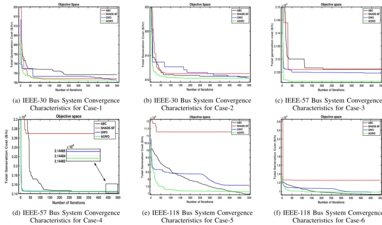
The objective of Case-1 is to optimize the power gener-ation schedule of all RES and TPGs to reduce total power generation cost using Eq. 23. For illustrative purposes, the values of direct, reserve and penalty cost coefficients for WSH generation system ared= 1.6,r= 3 andp= 1.5, respectively. The total generation cost achieved by AGWO is 781.13 $/h and that of GWO is 781.77 $/h shown in Table IV. These results are compared with the results obtained from ABC and SHADE-SF algorithms, i.e., 784.24 $/h and 782.82 $/h. More details about these algorithms can be found in Refs. [2] and [4]. Fig. 1a shows that AGWO has faster convergence and less computational time than the other three algorithms.

(5)

0 50 100 150 200 250 300 350 400 450 500 Number of Iterations 780 785 790 795 800 805 810 815 820

Total Generation Cost ($/hr)

Objective Space

ABC SHADE-SF GWO AGWO

(a) IEEE-30 Bus System Convergence Characteristics for Case-1

0 50 100 150 200 250 300 350 400 450 500 Number of Iterations 810 815 820 825

Total Generation Cost ($/hr)

Objective Space

(b) IEEE-30 Bus System Convergence Characteristics for Case-2

0 50 100 150 200 250 300 350 400 450 500 Number of Iterations 2.125 2.13 2.135 2.14 2.145 2.15

Total generation cost ($/h)

104 Objective space

(c) IEEE-57 Bus System Convergence Characteristics for Case-3

0 50 100 150 200 250 300 350 400 450 500 Number of Iterations 2.14 2.16 2.18 2.2 2.22 2.24 2.26 2.28 2.3

Total Generation Cost ($/h)

104 Objective space ABC SHADE-SF GWO AGWO 2.14483 2.14484 2.14485 104

(d) IEEE-57 Bus System Convergence Characteristics for Case-4

0 50 100 150 200 250 300 350 400 450 500 Number of Iterations 7 7.5 8 8.5 9 9.5 10 10.5 11 11.5 12

(e) IEEE-118 Bus System Convergence Characteristics for Case-5

0 50 100 150 200 250 300 350 400 450 500 Number of Iterations 1 1.2 1.4 1.6 1.8 2 2.2 2.4 2.6

(f) IEEE-118 Bus System Convergence Characteristics for Case-6

Fig. 1:Convergence Characteristics of AGWO and Recent Techniques for Case-1–Case-6.

TABLE IV: Comparison Between AGWO and other Algorithms for IEEE-30 bus System using Case-1 and Case-2.

Case-I Case-II

Min Max (ABC) (SHADE-SF)[4] (GWO) (AGWO) (ABC) (SHADE-SF)[4] (GWO) (AGWO)

PT g,1(MW) 50 140 131.4 130.6 129.6 130.1 108.4 109.6 109.8 108.1 PT g,2(MW) 20 80 38.5 37.6 38.1 36.2 43.7 44.7 44.7 41.3 PW g,1(MW) 0 75 37.5 43.8 48.9 39.5 42.8 43.5 42.4 41.7 PT g,3(MW) 10 35 10.4 10 10 10 12.1 10.5 11.05 16.3 PW g,2(MW) 0 60 39.8 40.0 37.8 40.1 44.0 43.9 43.9 43.7 PSg(MW) 0 50 31.2 31.9 31.9 32.8 36.9 35.7 36 36.3 Total cost ($/hr) 784.24 782.82 781.77 781.13 813.81 811.43 810.17 810.15

Elapsed time (Seconds) 367 272 279 230 395 272 286 246

Carbon emission (ton/h) 1.42 1.35 1.28 1.48 0.7 0.58 0.42 0.39

B. Case 2: Optimizing Fuel Cost and Carbon Emission

The main objective of Cas-2 is to minimize total generation costs while imposing a carbon tax on the amount of carbon emission from TPGs. Total generation cost, including the carbon tax, is calculated with the help of Eq. 24. Carbon tax (Ctax) is considered at the rate of $20/ton [4]. The optimized generation schedule of all generators, total power generation cost, values of carbon emissions and other parameters for all algorithms are provided in Table IV. It is clearly depicted that RES contribution gets higher when the carbon tax is imposed in Case-2, compared to Case-1 (when there is no tax on carbon emission). The obtained result of emission gases by AGWO is 0.39259 ton/h, which is the lowest value compared with 0.42503 ton/h, 0.58487 ton/h and 0.7049 ton/h obtained by GWO, ABC and SHADE-SF, respectively, as given in Table IV. The convergence properties of AGWO, basic GWO and

other approaches is shown in Fig. 1b.

VII. CASE STUDIES FORIEEE-57BUS SYSTEM

The objective of Case-3 is to optimize the power generation schedule of three RES and TPGs to reduce total power generation costs in the IEEE-57 bus system. It is similar to Case-1 in the IEEE-30 bus system and the objective function of the quadratic fuel cost is given in Eq. 23. The total cost obtained by the AGWO algorithm is 21215 $/h, which hits the best minima in search space compared to the ABC, SHADE-SF and GWO. The fuel cost value by ABC is 21262 $/h, by SHADE-SF is 21260 $/h and by the GWO is 21247 $/h, as given in Table V. The convergence properties of AGWO and other optimization methods are shown in Fig. 1c.

(6)

TABLE V:Simulation Results for IEEE-57 Bus system using Case-3 and Case-4.

Bus System IEEE-57

Objective function ABC SHADE-SF [4] GWO AGWO

Case-3 Case-4 Case-3 Case-4 Case-3 Case-4 Case-3 Case-4

Cost (MW/h) 21262 21450 21260 22693 21247 21448 21215 21448

Carbon emission (ton/h) 33 16 39 23 36 10 31 9.42

Computational time (Sec) 870 448 330 298 247 255 220 243

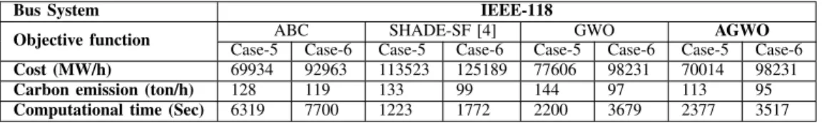
TABLE VI: Simulation results for IEEE-118 Bus System using Case-5 and Case-6.

Bus System IEEE-118

Objective function ABC SHADE-SF [4] GWO AGWO

Case-5 Case-6 Case-5 Case-6 Case-5 Case-6 Case-5 Case-6

Cost (MW/h) 69934 92963 113523 125189 77606 98231 70014 98231

Carbon emission (ton/h) 128 119 133 99 144 97 113 95

Computational time (Sec) 6319 7700 1223 1772 2200 3679 2377 3517

This Case study is conducted to optimize the OPF solution for quadratic fuel cost and carbon emission control for the objective function given in Eq. 24. It is evident from Table V that AGWO obtains the lowest values for this Case study with fuel cost and carbon emission values of 21448 $/h and 9.42 ton/h, respectively. The variation of total fuel cost between AGWO and other algorithms are shown in Fig. 1d.

VIII. CASE STUDIES FORIEEE-118BUS SYSTEM

In this Case study, the generation system total fuel cost minimization is taken as an objective function given by Eq. 23. The cost computed by AGWO for this Case is 70014 $/h, which is better than SHADE-SF and the original GWO [7], which are respectively 77606 $/h and 129509 $/h. The ABC algorithm achieves the minimum cost for this case study with an obtained value of 69934 $/h. Table VI provides obtained values comparison for generation costs, carbon emissions and computational time for all algorithms. The convergence graph in Fig. 1e reveals that AGWO has better convergence characteristics than GWO and other approaches reported in the literature.

Both quadratic fuel cost and emission gases minimization is the aim of this Case study. The objective function calculation is based on Eq. 24. With carbon tax imposition, the value of emission is significantly reduced from 113 ton/h in Case 5 to 95 ton/h. The ABC algorithm obtained lower costs for Case-5 and Case-6 but at the cost of computational time. The AGWO algorithm requires the least computation time, suggesting that it is a highly promising algorithm for industrial applications. Fig. 1f compares the convergence characteristics of all algorithms for 500 trial run.

IX. CONCLUSION

This paper presents a solution strategy for OPF study considering traditional TPGs and the intermittent nature of renewable energy sources (RES). Different PDFs were used to model WPG, SPG and HPG uncertainty, and their integration

methods were discussed. Several case studies were investigated to evaluate the performance of the proposed algorithm and the results were compared with other well recognized evolutionary algorithms. Hence, novel contributions include the proposed objective functions that consider RES; the use of an AGWO approach to address the non-convex OPF problem, and its ap-plication both in small, medium and higher-scale bus systems with evaluation via simulation.

The new results in this article show the AGWO proves to be very useful and reliable with a fast convergence rate to find a global solution for considered objective functions. It outperforms other algorithms in terms of total cost and convergence time minimization, whilst simultaneously addressing the necessary system constraints.

Acknowledgements The authors acknowledge funding support from COMSATS University Islamabad, Lahore campus and Lancaster University UK to support this project.

REFERENCES

[1] M.A. Taher, S. Kamel, F. Jurado and M. Ebeed, “Modified grasshopper

optimization framework for optimal power flow solution,” Electrical

Engineering, vol. 101, no. 1, pp. 121-148, Apr 2019.

[2] H. Jadhav and R. Roy, “Gbest guided artificial bee colony algorithm

for environmental/economic dispatch considering wind power,” Expert

Systems with Applications, vol. 40, no. 16, pp. 6385-6399, Nov 2013.

[3] S. S. Reddy and J. A. Momoh, “Realistic and transparent optimum

scheduling strategy for hybrid power system,” IEEE Transactions on

Smart Grid, vol. 6, no. 6, pp. 3114-3125, Mar 2015.

[4] P. P. Biswas, P . N. Suganthan and G. AJ. Amaratunga, “Optimal power

flow solutions incorporating stochastic wind and solar power,”Energy

Conversion and Management, vol 148, iss. 2017, pp. 1194-1207, Sep

2017.

[5] P. P. Biswas, P. N. Suganthan, B. Y. Qu, and G. AJ. Amaratunga, “Multiobjective economic-environmental power dispatch with stochastic

wind-solar-small hydro power,” Energy, vol. 150, iss. 2018, pp.

1039-1057, May 2018.

[6] S. S. Reddy, S. Surender, P. R. Bijwe and A. R. Abhyankar, “Real-time economic dispatch considering renewable power generation variability

and uncertainty over scheduling period,”IEEE System Journal, vol 9, no.

4, pp. 1440-1451, Jun 2014.

[7] S. Mirjalili, S. M. Mirjalili and A. Lewis, “Grey wolf optimizer,”

Advances in Engineering Software, vol 69, iss. 2014, pp. 46-61, Mar

2014.

[8] M. H. Qais, H. M. Hasanien, and S. AlghuwainemM, “Augmented grey wolf optimizer for grid-connected PMSG-based wind energy conversion

systems,”Applied Soft Computing, vol 69, iss. 2018, pp. 504-515, Aug