A comparison of supervised learning algorithms

A comparison of supervised learning algorithms

First Examiner: Prof. Dr. Wolfgang Härdle

Second Examiner: Prof. Weining Wang

Thesis Supervisor: Dr. rer. nat. Sigbert Klinke

In partial fulfillment of the requirements for the degree of

Bachelor of Science (B.Sc.) in Economics

Table of contents

1 Introduction……… ………

1

2 Data……… ………..

3

2.1. Data preparation ……….……… 3

3 Methods...

5

3.1. Classification and Regression Trees CART……… 5

3.1.1. Construction of the classification tree ..……….. 5

3.1.2. Gini splitting rule ………..……… 7

3.1.3. Minimal cost-complexity pruning ………..……… 7

3.2. Multiple logistic regression ……… 8

3.2.1. Introduction to the multiple logistic regression ………..………… 8

3.2.2. Fitting the logistic regression model ……….……….. 9

3.2.2. Interpretation of the regression coefficients ……….……. 10

3.3. Naive Bayes Classifier ………. 11

3.4. Feedforward neural network …... 12

3.4.1. Multilayer networks and the backpropagation algorithm ..…………. 12

3.4.2. Universal approximation theorem ……….…….….. 13

3.4. Feedforward neural network …... 14

3.4.1. Confusion matrix ..………..……. 14

3.4.2. ROC Analysis and AUC ……….…….………….… 15

4 Analysis

...

17

4.1. CART ..……….……… 17

4.1.1. Constructing the classification tree ..……….….……….. 17

4.1.2. Tree selection ……….……..………… 19

4.2. Multiple logistic regression ……….……… 19

3.2.2. Fitting the logistic regression ……….……….…….. 20

4.3. Naive Bayes Classifier ………. 25

4.4. Feedforward neural network ……… 27

4.4. Final comparison ………..……… 29

5 Discussion

...

31

6 References

………..………

33

List of Tables

3.1. Confusion matrix ……….… 14

4.1. AUC measures of different classification tree versions ………..……. 19

4.2. Correlation matrix ……….…….….……. 20

4.3. Results of the initial logistic regression ……….….………. 21

4.4. Results of the stepwise backward logistic regression model ……….….……. 22

4.5. AUC scores of the two logistic regression models ……….………. 22

4.6. Logistic regression thresholds ……….……….…….. 24

4.7. AUC scores of the Naive Bayes classifiers ……….…..…. 27

4.8. Results of the random search for the hyperparameters ……….…. 29

4.9. Final comparison ………..……….……. 29

List of Figures

4.1. Visual representation of the relationship between the pruned tree size, the corresponding complexity parameters and the cross-validated misclassification error ………. 17

4.2. Classification tree based on the default pruning rule from rpart command in R .…….. 18

4.3. ROC curves of the two logistic regression models ……….….…..……. 24

4.4. ROC curves of the stepwise logistic regression model with different thresholds .……. 25

4.5. Histograms of the two numeric variables in the PUMS dataset ……….………. 26

4.6. Logistic regression thresholds ……….……….…….. 27

1 Introduction

The fields of machine learning and computational statistics have gained a lot of attention in the last years, and every now and then buzzwords like “Artificial Intelligence” and “Predic-tive Models” get mentioned in news (e.g. The Economist, 2016). It is not surprising, since machine learning algorithms have become crucial tools for improving products of many com-panies in various industries. Especially nowadays, when the amounts of data available are lar-ger than ever before, it is easier for analysts to gain new insights and to perform analyses that are not limited by the scarcity of data. Thus, it is a natural consequence that certain methods and algorithms, which were created before the universal increase in computational powers and digital upheaval in many industries, are used more than ever before.

However, while there are also a lot of the statistical and machine learning tools and methods used, it may be sometimes unclear which method should be used on a specific task. From my own experience working in an IT company with a strong analytical team, it can happen that personal preference of an analyst plays bigger role than a deliberated decision, when it comes to choosing the suitable method for a given task. As a matter of fact, it is often hard to say be-forehand, whether the results of different methods applied will be different. But the conse-quences of applying the wrong tool may be incorrect future decision making and, potentially, a loss of potential revenue of a company. Therefore, it is an important topic, which affects many businesses in a direct way.

It made me think, if the use of different methods would really make a significant difference in results within the framework of, for example, a binary classification task? How strong are the differences? Is there a single best supervised learning algorithm?

That is why the focus of this thesis lies on the comparison of results that are generated by the supervised learning algorithms. Since there are numerous supervised learning algorithms available nowadays, that can solve a binary classification problem, this thesis concentrates only on several algorithms, that are most widely known.

Most of the big companies with a lot of capital develop their own learning algorithms, howe-ver it is howe-very hard, if not impossible, to obtain those algorithms and compare them. They are also suited to specific needs of each company and thus make a comparison biased towards a certain task. Startups, in turn, may opt for the algorithms that are open to the public and that can be easily compared with each other.

It is important to note that the computational requirements and duration of the algorithms will not be the main focus of this thesis, despite the fact that they can play not the last role when choosing an algorithm in a business environment.

The binary classification task, that is going to be solved in the following analysis, is whether an American inhabitant earns more or less than 50 thousand dollars a year.

This thesis is organised as followed. Section two describes the dataset, which was used for the analysis, in detail. Section three contains the detailed description of algorithms that were cho-sen for the later analysis and comparison, and the section four describes the analysis and the results of it. Finally, section 5 summarises the thesis and attempts to give an answer to the questions stated above.

2 Data

For the purposes of this thesis, the American Community Survey (ACS) Public Use Microda-ta Sample (PUMS) of the year 2016 (one-year estimate) from the US Census Bureau was used. Each PUMS file represents a sample of actual responses to the ACS, which is an ongo-ing survey that provides vital information on a yearly basis about the American nation and its people, namely about jobs and occupations, educational attainment, veterans, whether people own or rent their homes, earnings and other topics. It was started in 2005 and replace once-a-decade census form that was decreasing overall census response rates and jeopardising the accuracy of the count (US Census Bureau, 2018).

ACS one-year estimates summarise responses received in a given year for all states and each record in the PUMS represents a single person. And since the 2016 PUMS contains data on approximately one percent of the United States population, it is a weighted sample that was drawn from the whole US population.

2.1. Data preparation

The initial PUMS file had more than three million observations and 284 variables. As mentio-ned in the introduction, the upcoming analysis will focus on earning of American inhabitants, hence it makes more sense to focus on those, who are able to earn money in the first place. The minimum age to work without any restrictions in every industry in the United States is 18 (U.S. Department of Labor, 2011), therefore individuals that are younger than 18 were remo-ved from the data set. Furthermore, a lot of variables in dataset are of no interest for the fur-ther analysis eifur-ther because fur-there is a lot of data missing in them, or they provide some speci-fic information about a more general variable, or there simply doesn’t seem to be a connection between those variables and someone’s ability to earn money. For example, variable “Veteran period of service” seems to show no connection to one’s earning on a grand scale and variable “Interests, dividends, and net rental income past 12 months” is redundant, when there is a va-riable “Total person’s income”.

Besides, the variable “Total person’s income” (PINCP), which is a target variable in the fur-ther analysis, was transformed from a numeric to a binary variable with categories “earned less than 50 thousand dollars (<50k)” and “earned at least 50 thousand dollars (>=50k)”. The variable “Educational attainment” (SCHL) was also recoded into a variable “school” in order

to reduce the number of classes and remove empty ones. The same applied to the variable „Marital status“ (MAR).

It means that the dataset, which will be analysed further, has ca. 2.5 million observations and ten variables. The full list and description of the customised variables used in the analysis can be found in Appendix.

The dataset was also split into three sets with a 60/20/20 split – a training set, a validation set and a test set respectively. The observations were drawn randomly, which ensure that the dis-tribution of the data in each set of the data is equal to each other.

2.1.1. Missing values

Luckily, the dataset had almost no missing values, or the NAs had a specific meaning to them, which made it possible to put them in a separate category. For example, NAs in the variable „Class of worker“ meant that the person was not in labor force and it last worked five years ago or that it was never employed. Thus, the NAs were recoded as a separate category. The similar applied to the variable „Usual hours worked per week past 12 months“. There the mis-sing values meant that the person did not work past twelve moths and thus were recoded as numeric „0“.

The only true missing values were in the variable „school“. In the initial full PUMS file, NAs in the variable „school“ meant that the person is less than three years old. After removing people younger than eighteen years old, this doesn’t explain the missing values anymore. The-re weThe-re only 70 thousand missing values, which makes up only about two percent of the who-le sampwho-le size. Therefore, these cases were simply removed form the dataset, since such a small percentage is not significant for the further analysis.

3 Methods

3.1. Classification and Regression Trees (CART)

Classification and regression trees is a non-parametric decision tree learning algorithm that produces either a regression or a classification tree, depending on whether the dependent va-riable is categorical or numeric, respectively. It also can handle both continuous and categori-cal predictors. Since its first introduction by Breiman et al. (1984), CART appeals to many researchers and analysts due to its non-strict requirements and ease of interpretation.

CART algorithm is designed to represent decision rules in a form of binary trees, in which only only yes/no questions are asked, i.e each node has only two branches. Starting from the root node, all available variables and their possible values are looked through in order to find the split s – a combination of a variable from the available data and the appropriate question value. An optimal split s* is the one that maximizes homogeneity (i.e. reduces variance) insi-de the two subsets that result from splitting. The process is iterated for each of the subsets un-til the tree reaches its optimal size. The bottom of the tree is represented by terminal nodes, which constitute the final decision rule T*. (Andriyashin et al., 2008)

3.1.1. Construction of the classification tree

In the learning sample for a J class problem, let ! be the number of observations in class j. The priori class probabilities can then be defined as proportion of the classes in the populati-on:

where ! .

Similarly, ! is the number of observations in the node t, and ! is the amount of class j

observations in the node t. The probability that an observation of class j will fall into node t is given as: N_j (3.1.1) ! π(j) = N_Nj j = 1,...,J N(t) N_j(t) (3.1.2) ! p(j,t) = π(j)N_Nj(t) j

From here it follows that ! . Now we can derive that the conditional probabili-ty that an observation falls into node t, given its class j, is:

In other words ! are the relative proportions of class j observations in node t (Breiman et al., 1984).

As mentioned above, the classification tree is built in accordance with a splitting rule - a rule that determines split s* at each node. The goal is to create two more homogenous groups by splitting the initial less homogenous one (the parent node ! ) into two parts – left and right child nodes ! and ! . The split s* contains one variable ! from the matrix of explanatory va-riables ! (! where p is the number of observations in the learning sample) and a question value ! . A question „Is ! ?“ then splits the data. (Andriyashin et al., 2008) Homogeneity in a node is calculated with help of the the impurity measure ! , which is de-termined by the impurity function ! :

Then the goodness of split s can be measured as a reduction in impurity at the node t:

where ! and ! are proportions of observations that fall into ! and ! respectively. (Breiman et al., 1984)

Therefore, at each following node the following problem is solved:

The maximum tree ! is the tree containing the maximum number of nodes for a given data set. In other words, it is a tree built by applying equation (3.1.6) to the original data set and resulting split data portions until the following condition holds. This condition defines ! as the tree where each terminal node contains only observations belonging to the same class j:

where ! is the set of terminal nodes of a tree T.

p(t) =_∑ j p(j,t) (3.1.3) ! p(j|t) = p_p(₍j_t,₎t) = N_Nj₍(_tt₎) p(j,t) t_P t_L t_R x_i X X =X₁, . . . ,X_p x* x_i< x* i(t) ϕ(t) (3.1.4) ! i(t) =ϕ[p(1|t),p(2|t), . . . ,p(J|t)] (3.1.5) ! Δi(s,t) = i(t)−p_Ri(t_R)−p_Li(t_L) p_R p_L t_L t_R (3.1.6) ! s* = arg max

s Δi(s,t) = arg maxs [−pLi(tL)−pRi(tR)] = arg mins [pLi(tL) +pRi(tR)]

T_MAX TMAX (3.1.7) !∀t ∈T˜ ∃j :p(j|t) = 1 ˜ T

The next important step is to define the impurity function ! . Many different impurity func-tions can be used, but two of the most commonly used for CART are Twoing and Gini split-ting rules. According to Breiman (1996) all criteria should produce similar results, when the number of values of the dependent variable small. Since the dependent variable in the further analysis has only two values, any criteria could be chosen. Thus, Gini splitting rule was the rule of choice.

3.1.3. Gini splitting rule

Gini impurity is a measure of how often a randomly chosen observation from the set would be incorrectly classified, if it was randomly classified, according to the class distribution in the sample. It can be defined as:

The splitting rule employing the Gini impurity (derivation from (3.1.5)) can be written down as:

and (3.1.6) then takes the following form (Andriyashin et al., 2008):

3.1.3. Minimal cost-complexity pruning

Another important decision to make, when using classification trees, is to determine an opti-mal size of the tree. A maximum tree may be a good way to explain existing patterns in the available, but it is overfitted, when it comes to making predictions on an unknown set of data. On the other hand, a small tree may be not specific enough and also have a larger out-of-sample error, since it can’t classify precisely enough. One possible solution for this problem, proposed by Breiman et al. (1984) is cost-complexity pruning.

ϕ(t) (3.1.8) ! i(t) = 1−_∑J j=1 p2_(j|t) (3.1.9) ! Δi(t) =−_∑J j=1 p2_{(j|t) +p} L J ∑ j=1 p2_(j|t L) +pR J ∑ j=1 p2_(j|t R) (3.1.10) ! s* = arg max s [− J ∑ j=1 p2_{(j|t) +p} L J ∑ j=1 p2_(j|t L) +pR J ∑ j=1 p2_(j|t R)]

The cost-complexity measure of a tree is defined as:

where ! is any subtree of the maximum tree, R(T) is the misclassification cost, or the internal misclassification error of the tree, ! is the number of terminal nodes, or com-plexity of the subtree, and ! is the complexity parameter.

While ! can take on an infinite number of values, there is only a finite number of subtrees of a maximums tree. Therefore, if there is an optimal tree for a given ! , it will remain optimal, unless ! will change.

The optimal subtree ! is defined by the conditions: (i) !

(ii) If ! , then !

The result of this pruning is a sequence of subtrees ! {! }, where {! } is the root node, for which the sequence of alphas, {! }, is increasing. By applying the method of V-fold cross-validation to the sequence of subtrees, an optimal tree can be determined.

However, selecting a tree with the minimum value of ! is not always the best choice, because usually the whole range of ! which satisfy ! < ! for small ε > 0. Besides, running a V-fold cross-validation procedure might give slightly different results. Thus, a so called one standard error rule can be applied, according to which a value of ! within one standard error can be chosen (Andriyashin et al., 2008)

3.2. Multiple Logistic Regression

Multiple logistic regression represents one of the regression analysis methods. It describes the relationship between a binary or dichotomous variable Y and multiple explanatory variables denoted by X, which represents the whole set of independent variables ! . The dicho-tomous response variable is what makes the multiple logistic regression model different from the standard multiple regression model.

3.2.1. Introduction to Multiple Logistic Regression

In the logistic regression, the conditional mean (mean value of the outcome variable, given the values of the independent variables), expressed as ! , can only be greater than or (3.1.11) ! R_α(T) = R(T) +α|T˜| T ≤T_MAX |T˜| α ≥0 α α α T(α) Rα[T(α)] = min_T≤T MAXRα(T) Rα(T) = Rα[T(α)] T(α) ≤T T1>T2> . . . > t1 t1 αk RCV_(T) RCV_{(T) R}CV_{(T) R}CV min(T) +ε ̂ RCV_(T) x₁, . . . ,x_k E(Y|X)

equal to zero and less than or equal to one (i.e. ! ), compared to the multiple regression model, where the conditional mean ranges between ! and ! . The reason for this is that a probability can’t be greater than one or less than zero. Thus, the conditional mean follows an S-shaped distribution, which is given by the logistic function.

In order to simplify notation, the conditional mean ! is further denoted as ! , and it is calculated as:

Besides, the conditional distribution of the outcome variable given X is not normal with mean ! , and the variance is not constant. In the case of dichotomous outcome variable, the outcome variable can be expressed as ! . Here the quantity ε may assume one of two possible values. If ! then ! with probability ! , and if ! then ! with probability ! . Thus, ε has a distribution with mean zero and vari-ance equal to ! . That is, the conditional distribution of the outcome variable follows a binomial distribution with probability given by the conditional mean, ! (Hos-mer et al., 2013).

Since the dependent variable in the logistic regression follows the Bernoulli distribution, the independent variables need to be linked to the Bernoulli distribution (or binomial distribution with n = 1 trials). In order to accomplish this, a link function called ‘logit’ is used.

The logit transformation of ! is defined in terms of ! as:

Now the probability of an event occurring or not is converted into a continuous variable that is linear with respect to the explanatory variables. ! is also called log-odds of an event occurring (or not occurring).

3.2.2. Fitting the Logistic Regression Model

The regression parameters in the logistic regression are estimated with help of the maximum likelihood method. In general sense, it yields values for the unknown parameters that

maximi-0≤ E(Y X) ≤1 −∞ +∞ E(Y|X) π(X) (3.2.1)

!

π

(

X

) =

e

1 +

e

se the probability of obtaining the observed set of data. In order to apply this method, a func-tion that expresses probability of the observed data as a funcfunc-tion of unknown parameters (li-kelihood function), is needed in the first place. Afterwards, maximum li(li-kelihood estimators (MLE) of the parameters need to be calculated. They maximise the likelihood function, hence they agree most closely with the observed data (Hosmer et al., 2013). Here is how those va-lues are found:

The conditional probability of ! , given X is denoted as ! otherwise ! . Therefore, for the pairs ! where ! is the value of the inde-pendent variable and ! is the value of the dependent variable for the !-th observation, the contribution to the likelihood function, when ! and ! are ! and 1 −! respec-tively. Therefore, the contribution of the pair ! to the likelihood function can be calcula-ted as:

As the observations are assumed to be independent, the likelihood function is given as:

where ! is a vector of parameters ! and ! is the number of observations.

Since it is easier to find values that maximize ! with the log of the equation (3.2.4), the log-likelihood is defined as:

Values of ! that are a result of solving the maximization problem in the equation 3.2.5 are the MLEs.

3.2.3. Interpretation of the regression coefficients

The regression coefficients in the logistic regression have also a different interpretation com-pared to the linear regression, because of the logit link function. In case of the categorical in-dependent variable, ! dummy variables need to be created for ! categories. Then, a regression coefficient represents the natural logarithm of the ratio of the odds that Y=1 among

Y = 1 P(Y = 1|X) =π(x), P(Y = 0|X) = 1−π(X) ₍xi,yi)  xi yi i yi= 1 yi= 0 π(xi) π(xi) (xi,yi) (3.2.3) ! π₍x_i)yi_[1−π (xi)1−yi]  (3.2.4) ! l(β) = _∏n i=1 π₍x_i)yi_[1−π (xi)1−yi] β β₀, β₁, …, β_k n β (3.2.5) ! L(β) = ln[l(β)] =_∑n i=1{ yiln[π(xi)] +(1−yi)ln[1−π(xi)]} β k −1 k > 2

observations of a certain category to the odds of Y=1 among observations of the left out, or reference, category:

where ! is the reference category, and ! is one of the categories (Hosmer et al., 2013). A continuous dependent variable, on the other hand, shows the difference in the log odds, when the continuous dependent variable increases by one unit.

3.3. Naive Bayes classifier

Naive Bayes classifier is a simple but very practical and useful Bayesian learning method. Its approach to classifying data is to assign the most probable target value, ! (MAP = Maxi-mum A Posteriori), given the attribute values ! that describe the instance.

Applying the Bayes theorem to this expression gives us:

However, estimating various ! terms is complicated as the dimensionality increases. Therefore, the naive Bayes classifier utilises one simplifying assumption. It assu-mes that the attribute values ! are conditionally independent, given the target value. So given the target value ! , the values of different attributes do not affect each other, i.e. the probability of observing the conjunction ! is just the product of the probabilities for the indi-vidual attributes, which gives us:

where ! is the target value predicted by the naive Bayes classifier. Whenever the assumpti-on of cassumpti-onditiassumpti-onal independence is satisfied, ! is identical to ! (Mitchell, 1997).

(3.2.6) !

OR

=

=

=

e

vMAP = arg max_v

j∈V P(vj|a1,a2, . . . ,an)

(3.3.2)

!

vMAP = arg max_v

j∈V P(a₁,a₂, . . . ,a_n|v_j)P(v_j) P(a1,a2, . . . ,an) = arg maxvj∈V P(a1,a2, . . . ,an|vj)P(vj) P(a₁,a₂, . . . ,a_n|v_j) ai vj a1,a2, . . . ,an (3.3.3) ! vNB= arg max_v j∈V P(vj)∏_i P(ai|vj) v_NB v_NB v_MAP

3.4. Feedforward neural network

While nowadays there are many different types of artificial neural networks (ANNs), this the-sis focuses only on the simplest type – the feedforward neural network.

Simply put, the concept of ANNs was inspired by the basic fact that the biological learning systems in the animal and human brains consist of interconnected neural webs. ANNs remote-ly resemble them, in that they’re built out of an interconnected set of nodes, or artificial neu-rons, which each neuron can produce some kind of an output from a given input. This output can be then transmitted to the next layer of neurons, and so on.

The feedforward neural network has a structure of an acyclic graph, meaning that there are no cycles or loops. When data is „fed“ to the network, it moves only in one direction, forward, from the input node to the output nodes. Meanwhile, the network can have either none or multiple hidden layers between the input and the output layers. If a network has no hidden layers, it is called „perceptron“. This type of networks, however, is limited in its usage, since it utilises a step activation function (a function that defines the output of a node, given the in-put:

Where ! is the output, ! is an input and ! is a weight that determines the contri-bution of ! to the output.

It follows that while the perceptron can represent many primitive boolean functions like AND and OR, it fails to represent such functions like XOR (exclusive OR). In other words, the per-ceptron fails to learn not linearly separable patterns, i.e. that can not be correctly classified with a straight line (Mitchell, 1997). Therefore, using the multilayer perceptron (MLP), that has at least one hidden layer, is advised, in order to address possible non-linearities in the data.

3.4.1. Multilayer networks and the backpropagation algorithm

Multilayer networks are able to depict nonlinear nonlinear patterns, compared to the percept-ron. The weights for a multilayer network are learned by the backpropagation algorithm. It utilises gradient descent for minimisation of the error between the network output values and the target values from training data for these outputs. Gradient descent looks through the

hy-(3.4.1)

!

o(x1, . . . ,xn) =_{−1_{1 otherwise}if ω1x1+ . . . +ωnxn> 0

o(x1, . . . ,xn) xi ωi

pothesis space of possible weight vectors to find the weights that best fit the training exam-ples by the training error (Mitchell, 1997). The training error for a multilayer classification network is defined as:

with C representing the amount of classes, ! denoting weight of the input from node i to hi-dden unit j, ! denoting weight of the connection between a hidden and an output unit, ! being an activation function, ! if observation i belongs to class j and otherwise ! . The essence of the backpropagation algorithm can be captured as:

where t is the time parameter that separates different steps of the gradient descent search, ! is a positive constant called learning rate with ! , ! denotes weight of the input from node i to hidden or output unit j. The role of the learning rate is to moderate the degree to which weights are changed at each step of gradient descent.

Sometimes the weights are made to decay to avoid overfitting. Each weight is decreased by some factor during each iteration of the backpropagation algorithm, thus large weights in the network are penalised. Smaller weights smooth out the activation function and makes it more linear. Weight decay can be formally captured as:

where ! is the decay parameter (Klinke, 2018).

3.4.2. Universal approximation theorem

As Cybenko (1989) has shown, any continuous function can be approximated by a neural network that has only one hidden layer, given a sufficient amount of the nodes in this hidden layer. However, it is important to note that while a single hidden layer is sufficient, it may not be efficient, since the amount of nodes in the hidden layer, that can be required to yield some approximations may be quite high.

(3.4.2) ! EC =_∑ i=1 C ∑ j=1 yijlog[ N ∑ j=1 ωjΛωi0+ p ∑ i=1 ωijxi)] ω_ij ω_j Λ y_ij = 1 y_ij = 0 (3.4.3) ! ωij,t =ωij,t−1−λt_∂∂_ωE ij λ_t lim_t→∞λ_t = 0 ω_ij (3.4.2) ! E′=E+w(_∑ω2 j +_∑ωij2) w ∈[0,1]

According to Hornik (1991), this universal approximation property of the feedforward neural networks is achieved because of the feedforward property of the networks and not the choice of the activation function. Therefore, any non-constant, bounded, and monotonically increa-sing continuous activation function can be chosen.

3.5. Performance evaluation metrics

3.5.1. Confusion matrix

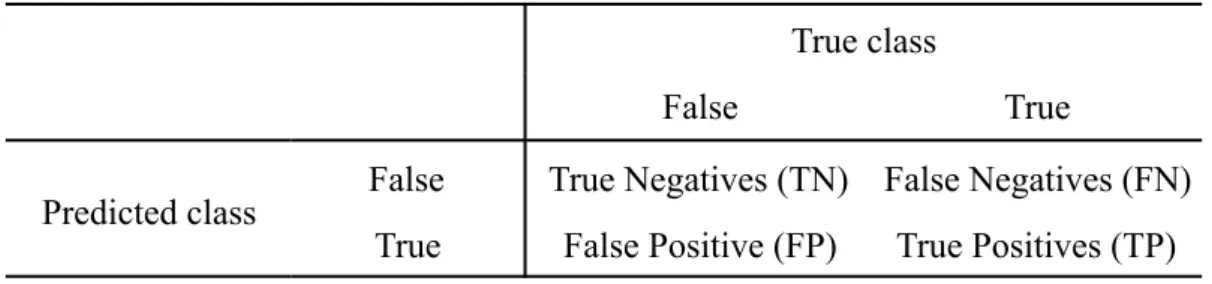
In order to compare different classification methods, some kind of a performance metric is needed. Since this analysis deals with a comparison of binary classifiers, metrics that are deri-ved from confusion matrix can be helpful. The confusion matrix represents four possible out-comes of a binary classification task: True Positives, False Positives, True Negatives and Fal-se Negatives, as shown in Table 3.1:

Table 3.1: Confusion Matrix

The true positives and the true negatives are observations, that are correctly classified by the classifier, whereas false positives and false negatives represent type I and type II errors re-spectively. In our classification task false positives would include people, who are classified as earning more than 50 thousand dollars per year, but are actually earning less than 50 thousand dollars. False negatives, on the other hand, are people, who are classified as earning less than 50 thousand dollars a year, but are actually learning more than 50 thousand dollars. The share of true positives and negatives in the whole set of predictions is defined as accura-cy:

Another metrics are recall (True Positive Rate):

True class

False True

Predicted class False True Negatives (TN) False Negatives (FN) True False Positive (FP) True Positives (TP)

(3.5.1)

!

and specificity (True Negative Rate):

While these metrics and other metrics similar to them can be used as tools to compare per-formance of classification models, they are easily influenced by class skewness (Fawcett, 2006). It means that they can show better performance of a model when the classes are ske-wed, compared to a case with balanced classes. For example, if a test dataset has 90% of ob-servations belonging to one class, and some classifier predicts that simply obob-servations be-long to that class, this classifier would still have high accuracy. Whereas if the classes were balanced, accuracy of this classifier would have been far worse.

3.5.2. ROC analysis and AUC

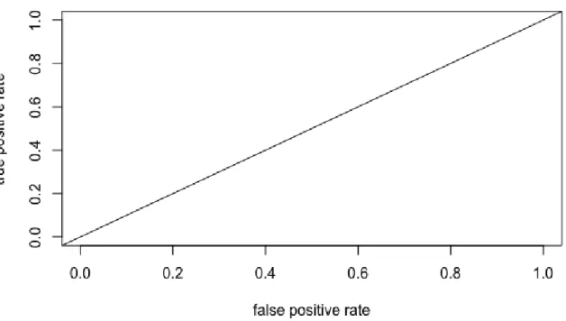
In such cases receiving operator characteristics (ROC) analysis is very helpful. ROC graphs are able to provide richer a richer measure of classification performance than scalar measures like accuracy, since they decouple classifier performance from class skew and error costs (Fawcett, 2006).

ROC graphs are two-dimensional graphs where the y-axis depicts true positive rate (precisi-on) and the x-axis depicts false positive rate (1 - specificity). Alternatively, the x-axis can also represent specificity with values condescending from one to zero. The ROC space is shown in Figure 3.1. If an ROC curve reaches point (0,1) in Fig. 1, it represents the perfect classifier. Thus, the more northwest an ROC curve reaches, the better the classifier is. The diagonal line illustrates random performance. Basically, such classifier predicts correct values 50% of the time. Any classifiers mapped on the right from the diagonal lines are showing worse than ran-dom performance, which makes them bad classifiers.

Area under the ROC curve (AUC) summarises the ROC performance in a single scalar, which allows for a simpler comparison of classification models. AUC is always between 0 and 1. The value of 0.5 represents the area under the diagonal line in the ROC space, thus making . Besides, AUC has an important statistical interpretation: it is equivalent to the probability that (3.5.2) ! recall = _TPTP_+FP (3.5.3) ! specif icit y = _TNTN_+FN

the classifier will rank a randomly chosen positive instance higher than a randomly chosen negative instance, assuming that "positive" ranks higher than „negative“ (Fawcett, 2006). Because of its benefits and ease of interpretation, the AUC measure will be used in the further comparison of binary classification.

4 Analysis

The first supervised learning algorithm that was applied to solve the binary classification pro-blem, stated in the beginning, was the CART algorithm.

4.1. CART

4.1.1. Constructing the classification tree

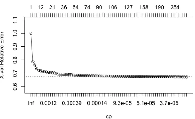
Firstly, a maximum tree was grown, using the data from the training set. The result is a huge tree with more than thirteen thousand terminal nodes, where all the variables were used. After applying cost-complexity pruning with ten-fold cross-validation, the tree size reduced con-siderably, but it still remained quite large with 439 terminal nodes. Therefore, the one stan-dard error rule was applied, in order to further reduce the size of the classification tree. The amount of terminal nodes now reduced down to 303. However, as one can see in the Figure 4.1, there is not much improvement happening, associated with the misclassification error, when the size of the tree increases after a certain point.

Figure 4.1: Visual representation of the relationship between the pruned tree size, the corre-sponding complexity parameters and the cross-validated misclassification error.

Moreover, many of the terminal nodes have 50 to 300 observations, which is negligible, ta-king into account that the training set contains almost 1.5 millions of observations.

It was also interesting to see, if the default rpart procedure in R would deliver different re-sults, therefore a decision tree with default pruning rule was also computed. The default rpart rule is that any split that does not decrease the internal misclassification error by a factor of the complexity parameter, will not be added to the tree.

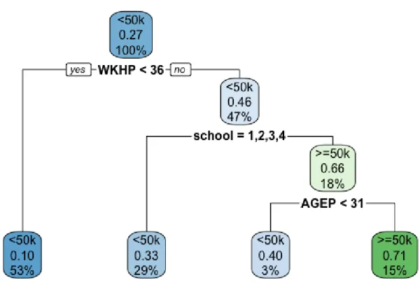
The results are indeed different, since the tree became considerably smaller and it uses only three variables out of twelve – Age, Hours worked per week and Educational attainment. Be-sides, it was possible to plot the tree itself (Figure 4.2) so that it would be descriptive enough for a reader. It makes use of one of the main advantages of the decision trees, i.e. ease of in-terpretability.

Figure 4.2: Classification tree based on the default pruning rule from rpart command in R There are no surprising results in the decision rules. It is intuitive that if one works more hours, has a better education and is older (because it is often correlated with working experi-ence), one will probably earn more money.

Next step is to see which tree predicts the annual income more accurate and choose one of them for the further comparison.

4.1.2. Tree selection

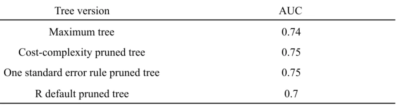
As described before, in order to select a tree for a further comparison with other algorithms, the AUC scores were compared. The performance of the trees was tested on a previously un-seen validation set of the data. This ensures that the out-of-sample error is taken into account. The results are shown in the Table 4.1:

Table 4.1: AUC measures of different classification tree versions

The results show that it would be best to choose the cost-complexity pruned tree with one standard error rule applied to it, since it has the same accuracy as the one without the one standard error rule, but is less complex.

It is worth to note that the difference between the AUC of this tree and the one that was prun-ed with default R pruning is 0.05, while the difference in the tree size is enormous. The R de-fault pruned tree provides the best AUC-size ratio by far, and it is way easier to interpret. However, since the emphasis of this thesis lies on the comparison of prediction power of dif-ferent algorithms and not on the interpretability, only the cost-complexity pruned tree will be considered in the further comparison.

4.2. Logistic regression

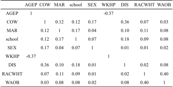
In order to build the logistic regression model, the independent variables needed to be firstly checked for multicollinearity to ensure stability and reliability of the estimated regression co-efficients. In case of numeric variables, the usual Pearson correlation coefficient was used, and the association between the categorical variables was measured with help of the Cramer’s V. The results are shown in Table 4.2:

Tree version AUC

Maximum tree 0.74

Cost-complexity pruned tree 0.75

One standard error rule pruned tree 0.75

Table 4.2: Correlation matrix

Fortunately, almost all of the independent variables have weak or very weak correlations bet-ween them. Therefore, there should be no reason for multicollinearity in the logistic regressi-on model, which would have drastically affected the regressiregressi-on coefficients.

Another preparatory step was to create ! dummy variables from nominal variables with ! categories, in order to be able to interpret the regression coefficients for these variables.

4.2.1. Fitting the logistic regression

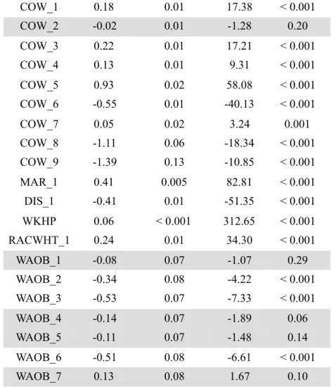
The results of the initial logistic regression are shown in Table 4.3. The dependent dummy variable is „Earns a person more than 50 thousand dollars per year?“. Value of 0 means no and 1 – yes. A number near the variable name indicates the category in the initial, non-dummy variable.

AGEP COW MAR school SEX WKHP DIS RACWHT WAOB

AGEP 1 -0.37 COW 1 0.12 0.12 0.17 0.36 0.07 0.03 MAR 0.12 1 0.17 0.04 0.10 0.11 0.08 school 0.12 0.17 1 0.07 0.18 0.09 0.08 SEX 0.17 0.04 0.07 1 0.01 0.01 0.02 WKHP -0.37 1 DIS 0.36 0.10 0.18 0.01 1 0.02 0.08 RACWHT 0.07 0.11 0.09 0.01 0.02 1 0.40 WAOB 0.03 0.08 0.08 0.02 0.08 0.40 1 k −1 k > 2

Estimate Std. Error z value Pr(>|z|) (Intercept) -4.12 0.08 -54.90 < 0.001 school_1 -3.00 0.02 -140.59 < 0.001 school_2 -2.45 0.02 -134.01 < 0.001 school_3 -1.93 0.02 -106.06 < 0.001 school_4 -1.57 0.02 -82.91 < 0.001 school_5 -0.87 0.02 -48.54 < 0.001 school_6 -0.29 0.02 -15.52 < 0.001 school_7 -0.08 0.02 -3.52 < 0.001 SEX_1 0.75 0.005 156.06 < 0.001 AGEP 0.04 < 0.001 241.37 < 0.001

Table 4.3: Results of the initial logistic regression

There are five insignificant variables in the initial logistic regression, which are marked grey. Insignificance means that the odds of Y=1 given the insignificant class is the same as of Y=1 given the reference class.

One possible solution for deciding which insignificant variables should be taken out of the model is a stepwise backward regression. In each iteration it deletes the variable with smallest partial correlation until the model becomes better (Klinke, 2018). The results of the stepwise regression are shown in Table 4.4.

COW_1 0.18 0.01 17.38 < 0.001 COW_2 -0.02 0.01 -1.28 0.20 COW_3 0.22 0.01 17.21 < 0.001 COW_4 0.13 0.01 9.31 < 0.001 COW_5 0.93 0.02 58.08 < 0.001 COW_6 -0.55 0.01 -40.13 < 0.001 COW_7 0.05 0.02 3.24 0.001 COW_8 -1.11 0.06 -18.34 < 0.001 COW_9 -1.39 0.13 -10.85 < 0.001 MAR_1 0.41 0.005 82.81 < 0.001 DIS_1 -0.41 0.01 -51.35 < 0.001 WKHP 0.06 < 0.001 312.65 < 0.001 RACWHT_1 0.24 0.01 34.30 < 0.001 WAOB_1 -0.08 0.07 -1.07 0.29 WAOB_2 -0.34 0.08 -4.22 < 0.001 WAOB_3 -0.53 0.07 -7.33 < 0.001 WAOB_4 -0.14 0.07 -1.89 0.06 WAOB_5 -0.11 0.07 -1.48 0.14 WAOB_6 -0.51 0.08 -6.61 < 0.001 WAOB_7 0.13 0.08 1.67 0.10 Null deviance 1,693,150 on 1,456,869 df Residual deviance 1,170,426 on 1,456,840 df AIC 1,170,486

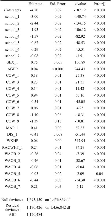
Table 4.4: Results of the stepwise backward logistic regression model

Now all the regression coefficients are significant on the significance level of ! = 5%. The regression coefficients also represent the expected tendencies, when it comes to the expected

Estimate Std. Error z value Pr(>|z|) (Intercept) -4.20 0.02 -187.12 < 0.001 school_1 -3.00 0.02 -140.74 < 0.001 school_2 -2.44 0.02 -134.15 < 0.001 school_3 -1.93 0.02 -106.12 < 0.001 school_4 -1.57 0.02 -82.92 < 0.001 school_5 -0.87 0.02 -48.53 < 0.001 school_6 -0.29 0.02 -15.51 < 0.001 school_7 -0.08 0.02 -3.51 < 0.001 SEX_1 0.75 0.005 156.89 < 0.001 AGEP 0.04 < 0.001 244.47 < 0.001 COW_1 0.18 0.01 25.38 < 0.001 COW_3 0.23 0.01 21.35 < 0.001 COW_4 0.14 0.01 11.42 < 0.001 COW_5 0.94 0.01 65.10 < 0.001 COW_6 -0.54 0.01 -45.05 < 0.001 COW_7 0.06 0.01 4.25 < 0.001 COW_8 -1.10 0.06 -18.31 < 0.001 COW_9 -1.39 0.13 -10.81 < 0.001 MAR_1 0.41 0.00 82.83 < 0.001 DIS_1 -0.41 0.008 -51.44 < 0.001 WKHP 0.06 0.00 347.94 < 0.001 RACWHT_1 0.24 0.01 34.29 < 0.001 WAOB_2 -0.26 0.04 -7.39 < 0.001 WAOB_3 -0.46 0.01 -38.67 < 0.001 WAOB_4 -0.06 0.01 -5.04 < 0.001 WAOB_5 -0.03 0.02 -2.09 0.04 WAOB_6 -0.44 0.03 -14.30 < 0.001 WAOB_7 0.21 0.03 6.12 < 0.001 Null deviance 1,693,150 on 1,456,869 df Residual deviance 1,170,426 on 1,456,842 df AIC 1,170,484 α

income. Each additional year of life and each additional working hour per week increases the odds of earning more than 50 thousand dollars per year by approximately four and six percent respectively. Furthermore, being disabled or not being in a marriage having a decreases the same odds. Moreover, the widely discussed facts that being a white male gives an advantage, when it comes to yearly earnings, are reflected in this model as well.

One interesting observation from this model is that being self-employed in own not incorpora-ted business (COW_6) gives worse odds of earning more than 50 thousand dollars per year than being not in labor force (COW_10, reference class).

4.2.2. Model selection

In order to see if the prediction power of the logistic regression was affected, the AUC scores of both models were compared on the validation set (Table 4.5). Both models have almost identical ROC curves and AUC scores, thus the stepwise backward logistic regression is pre-ferred because of the lesser complexity of the model.

Table 4.5: AUC scores of the two logistic regression models

Since the logistic regression does not make discrete predictions like CART does, ROC curves for both logistic regression models look smooth (Figure 4.3) and consequently have bigger AUC scores than the CART models. This occurs because the output of the logistic regression predicts probabilities of Y = 1 (! ) , and ROC curve shows the relationship between true and false positive rates for each classification threshold. It also means that predicting ac-tual classes requires a threshold for classification to be defined. It is a common practice to choose a threshold of 0.5, meaning that if ! > 0.5, Y = 1, and Y = 0 otherwise. In our case, Y = 1 means that a person earns more than 50 thousand dollars per year and Y = 0 means that a person earns less than 50 thousand dollars.

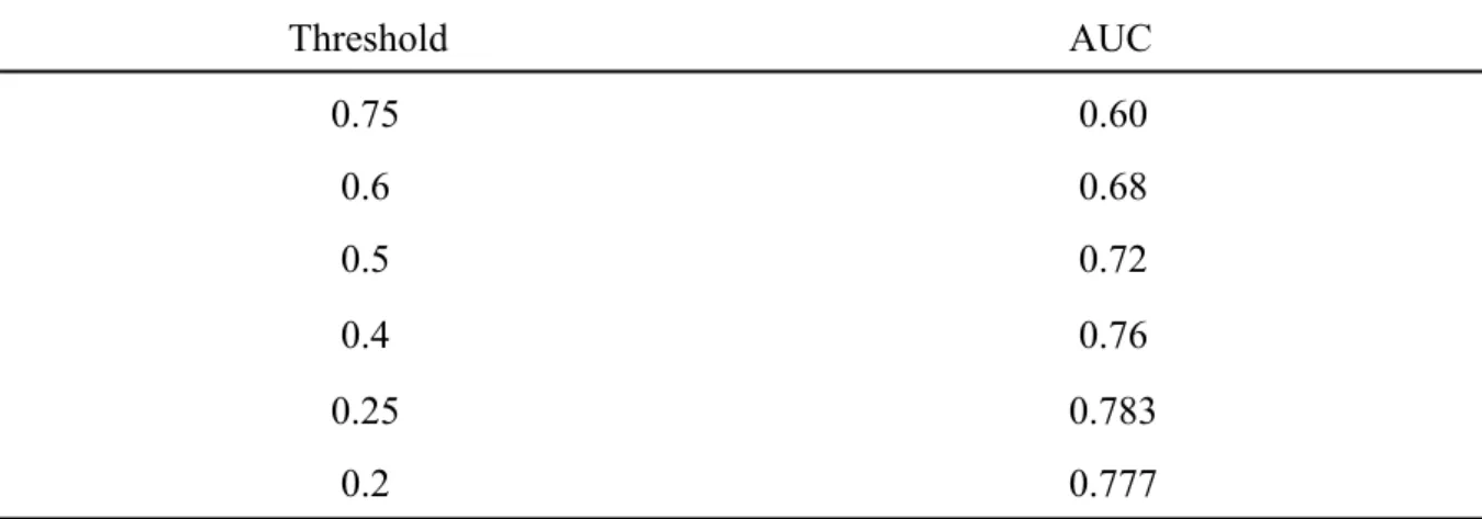
However, since the classes in our dataset are not balanced and the ratio between the classes is 75/25, a threshold of 0.5 might be not suitable. Therefore, other threshold values were also tested in order to see, whether their performance would be better. Table 4.6 shows that

thres-Logistic Regression Model AUC

Initial model 0.86

Stepwise backward model 0.86

Y= π(X)

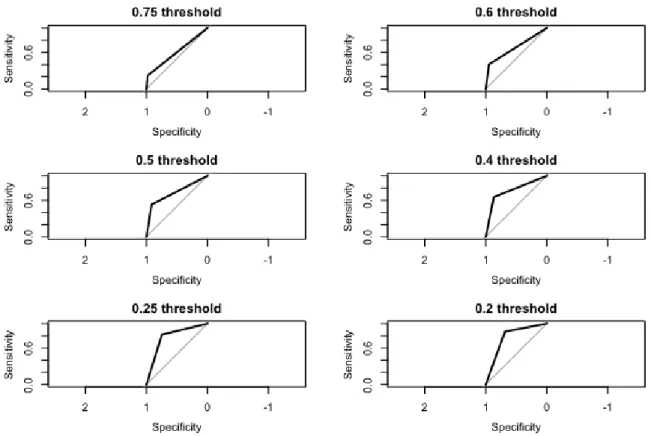
hold of 0.25 has the best performance, so it will be used in the following comparison. Figure 4.4 tells us that a smaller threshold allows for better sensitivity, on the cost of worse specifici-ty of the classifier.

Figure 4.3: ROC curves of the two logistic regression models

Table 4.6 : Logistic regression thresholds

Threshold AUC 0.75 0.60 0.6 0.68 0.5 0.72 0.4 0.76 0.25 0.783 0.2 0.777

Figure 4.4: ROC curves of the stepwise logistic regression model with different thresholds

4.3. Naive Bayes classifier

Naive Bayes classifier usually makes an assumption about continuous variables, that they fol-low a normal distribution, given the target class label (Ng and Jordan, 2001). In our dataset the numeric variables are definitely not normal distributed (Figure 4.5), however, they are not continuous, but discrete. Therefore, Naive Bayes can handle these discrete values as separate classes, which is one solution for not normal distributed continuous variables.

However, there are two another options – either to use kernel density estimation to estimate the class-conditional distributions, or recode the numeric variables into categorical variables. To be safe, all methods were tested and compared to each other.

The variable „Age“ was split into four categories, that attempt to resemble both life and working experience stages:

1) 18-30 years old – young adults, who just or recently entered the workforce and whose main focus is to gain experience and knowledge

Figure 4.5: Histograms of the two numeric variables in the PUMS dataset

2) 30-45 years old – middle-aged people, who can call themselves professionals and start to get higher positions

3) 45-60 years old – middle-aged, well-experienced workers 4) 60 years and older - senior people, mostly retired

The variable „Usual hours worked per week past 12 months“ was also split into four catego-ries:

1) 0 hours – did not work

2) 1-34 hours – part-time workers

3) 35-59 hours – usual working hours, full-time jobs

4) 60 hours and more – people who are working a lot of additional hours

All versions of the Naive Bayes classifier were then trained on the training set and their AUC scores were compared based on the validations set. The results are listed in the Table 4.7 and shown in Figure 4.6. As one can see, the version with kernel density estimation has a slightly better performance. Therefore, it will appear in the final comparison.

Table 4.7: AUC scores of the Naive Bayes classifiers

Figure 4.6: ROC curves of the Naive Bayes classifiers

4.4. Feedforward neural network

Training a proper feedforward neural network model required more preparation than other learning algorithms. First of all, the input data needed to be transformed. Categoric variables had to be transformed into dummy variables, like for the logistic regression. Furthermore, the numeric variables had to be normalised and brought into the range [0,1]. In order to achieve that, min-max normalisation was performed. It is defined as:

NB handling of continuous variables AUC

Kernel density estimation 0.7616

Categorization 0.75

Afterwards, a set of hyperparameters needed to be tuned. The simplest and most efficient way to do that is to perform a grid search over all of the hyperparameters and to see which combi-nation gives the best prediction power to the network. The parameters that were tested and compared were:

- The amount of gradient descent iterations/steps: 50, 100, 250, 500, 1000 - The amount of nodes in the single hidden layer: 3, 5, 10, 15, 20, 30, 40, 50 - Learning rate: 0.0001, 0.001, 0.01, 0.1

- Weight decay: 0.01, 0.1, 1

Different values for the amounts of gradient descent interactions and nodes in the hidden layer were chosen arbitrarily. The values for the learning rate were chosen according to a simple suggestion by Mitchell (1997), that it should be as low as possible. Weight decay values were chosen in accordance with Ripley and Venables (2004). The values for weight initialisation in the network were chosen as suggested by Marshald (2009) in the range between ! and ! , where n is the amount of input and hidden nodes in the network. Since different amounts of nodes in the hidden layer were tested, the average value was chosen, which means that the values for the initial weights were chosen from a range [-0.15, 0.15], and they followed uni-form distribution. Lastly, the tangent hyperbolic function was the chosen activation function. As on can see, there were 5x8x4x3 combinations of parameters to test. One way to accom-plish that was to perform a simple exhaustive search, where all combinations are tested against each other. However, it would require a lot of computational time. According to Berg-stra and Bengio (2012), random search is another effective solution, that allows to find mo-dels, that are as good as models configured by a pure full grid search, within a much smaller computational time. The random search can be optimized even more by defining early stop-ping criteria for the search. For this analysis, the early stopstop-ping criteria was to stop searching if the cross-entropy error has improved over the moving average of the best five models by less than 0.01. The results of the random grid search are shown in the Table 4.8:

(4.5.1) ! x′= _{ma x}x₍−_x)min_−min(x)_(x) − 1 n 1 n

Table 4.8: Results of the random search for the hyperparameters

The random search was stopped after the first five iterations, since the algorithm did not ob-serve a sufficient improvement in the cross-entropy error. The AUC score and the cross-en-tropy error were calculated on the validation set. The results show, that the differences in the five models are marginal. In order to balance out model complexity and predictive power, the model with 250 iterations, 10 hidden layers, learning rate of 0.1 and weight decay of 0.01 was chosen for the further comparison. The difference in the AUC to the „best“ model with the highest AUC is negligible, as well as in the cross-entropy error.

4.5. Final comparison

After the best models of all four supervised algorithms for a given dataset were defined, a fi-nal comparison on a test set of data could be carried out. The results are shown in Table 4.9 and Figure 4.7. Results show that in this analysis CART and Naive Bayes algorithms were outperformed by the logistic regression and feedforward artificial neural network. The latter two have almost the same AUC score, with logistic regression having a slight edge.

Table 4.9: Final comparison

Model Iterations Hidden Learning rate Weight decay AUC Cross-entropy

1 500 5 0.001 0.01 0.861 0.4026

2 250 5 0.1 1 0.862 0.4020

3 1000 5 0.01 0.1 0.863 0.3997

4 250 10 0.1 0.01 0.865 0.4027

5 100 30 0.1 0.1 0.866 0.3947

Supervised learning algorithm AUC

CART 0.7097

Logistic Regression 0.7851

Naive Bayes 0.7636

5 Discussion

By no means does this thesis represent an exhaustive empirical comparison of the four algo-rithms described before. Ideally, at least a couple more other supervised learning algoalgo-rithms should have also considered in the analysis. There was simply not enough time to test out all the possible models that could be created for those supervised methods. Nevertheless, the re-sults of the comparison in this thesis are congruent with a general consensus about the four algorithms analysed. The comparison has shown that different learning algorithms deliver si-gnificantly different results within the same classification problem.

When it comes to predicting binary outcomes, logistic regression or neural networks are first that come to mind, depending on the complexity of the task. Generally, they produce better predictions. This can also be observed in this thesis, since they both significantly outperform Naive Bayes and CART based on Area Under Curve measure.

Nevertheless, it does not mean that Naive Bayes or CART should be discarded, when it comes to building a predictive model. If one needs a white-box model, where the decision rules need to be retraced, decision tree is still one of the best options. Granted, the prediction errors will probably be higher, especially if the tree size needs to be reduced to increase comprehension. Naive Bayes is still often used, when it comes to e.g. natural language processing (Sang-Bum et al., 2006) thanks to its simplicity and robustness.

However, when it comes to predictions that have to be as precise as possible, ANN and logis-tic regression are more preferred. Areas that have such requirements are e.g. healthcare rese-arch and pharmaceuticals, and these areas use those algorithms for quite a while (Eftekhar et al., 2005). A study by Eftekhar et al., 2005 shows that in many cases artificial neural networks outperform logistic regressions. It makes sense, since neural networks are extremely flexible and if there is enough time for proper tuning of all of the hyperparameters, they most probab-ly deliver best results. However, artificial neural networks lack transparency in decision ma-king. Logistic regression offers both good predictive power and the ability to somewhat ex-plain what happens inside the model.

To sum up, a perfect supervised learning algorithm for solving a binary classification problem does not exist. Every algorithm has its up- and downsides, there are always traoffs. It de-pends on the goals of an analyst or a researcher, which algorithm will be used. Only when it comes to having solely best predictions possible, without the need to explain exactly why

tho-se predictions were made and there is enough time to develop it, one can say that artificial neural network is most certainly the best choice.

6 References

Andriyashin A., Härdle K. W., Timofeev R. (2008). Recursive Portfolio Selection with Deci-sion Trees. SFB 649 Discussion Paper 2008-2009, pp. 5-14.

Bergstra J., Bengio Y. (2012). Random search for Hyper-Parameter Optimization. Journal of Machine Learning Research 13, pp. 281-305.

Breiman L., Friedman H. J., Olshen A. R., Stone J. C. (1984). Classification and regression trees. Chapman & Hall, pp. 27-103.

Breiman L. (1996). Technical Note: Some Properties of Splitting Criteria. Machine Learning, Vol. 24, pp. 41-47.

Eftekhar B., Mohammad K., Ardebili E. H., Ghodsi M., Ketabchi E. (2005). Comparison of artificial neural network and logistic regression models for prediction of mortality in head trauma based on initial clinical data. BMC Med Inform Decis Mak, v. 5, https://dx.doi.org/ 10.1186/1472-6947-5-3.

Fawcett T. (2006). An introduction to ROC analysis. Pattern Recognition Letters 27, pp. 861-874.

Hosmer W. D., Lemeshow S. Jr., Sturdivant X. R. (2013). Applied Logistic Regression, Third Edition, pp. 1-61.

Klinke S. (2018), Slides from the lecture Data Analysis II.

Marshald S. (2009). Machine learning: an algorithmic perspective. Chapman & Hall/CRC, p. 58.

Mitchell M. T. (1997). Machine learning. McGraw-Hill, pp. 81–116.

Ng Y. A., Jordan I. M. (2001). On Discriminative vs. Generative Classifiers: A comparison of logistic regression and naive Bayes. Neural Information Processing Systems 2001, p. 2.

Ripley B. D., Venables W.N. (2002). Modern applied statistics with S, fourth edition. Sprin-ger, pp. 245-246.

Sang-Bum K., Kyoung-Soo H., Hae-Ching R., Sung H. M. (2006). Some Effective Techniques for Naive Bayes Text Classification. IEEE Transactions on knowledge and data engineering, vol. 18, no. 11, p. 1457.

The Economist (2017). Machine-learning promises to shake up large swathes of finance.

https://www.economist.com/finance-and-economics/2017/05/25/machine-learning-promises-to-shake-up-large-swathes-of-finance

U.S. Census Bureau (2018). About PUMS. https://www.census.gov/programs-surveys/acs/ technical-documentation/pums/about.html

U.S. Census Bureau (2018). About American Community Survey. https://www.census.gov/ programs-surveys/acs/about.html

U.S. Department of Labor (2011). The Fair Labor Standards Act of 1938. https://ww-w.dol.gov/whd/regs/statutes/FairLaborStandAct.pdf

7 Appendix

Coded variable name Description Variable type/variable values

AGEP Age Numeric; 1-99

COW Class Of Worker

Categorical; NA (10) -Not in labor force who last worked more than five

years ago or never worked, 1 - Employee of a private for-profit company or of an individual, 2 - Employee of a private not-for-profit

organization, 3 - Local government employee, 4 - State government employee, 5 - Federal government employee, 6 - Self-employed in own

not incorporated business, 7 - Self-employed in own not incorporated business, 8 - Working without pay in

family business or farm, 9 - Unemployed and last worked five years ago or earlier or never worked

MAR Marital status Categorical; 1 - Married, 2 - Not

married

school Educational attainment

Categorical; 1 - below HS diploma, 2 - HS diploma or similar, 3 - College

dropout, 4 - Associate's degree, 5 - Bachelor's degree, 6 - Master's degree, 7 - Professional degree beyond a bachelor's degree, 8 -

Doctorate degree

SEX Sex Categorical; 1 - male, 2 - female

WKHP Usual hours worked per week past 12 months

Numeric; 0 - did not work, 1-98 – 1 to 98 usual hours, 99 - 99 or more

DIS Disability Categorical; 1 - With a disability, 2 - Without a disability

income Total person’s income in the _{past 12 months}

Categorical; <50k - less than 50 thousand dollars, >=50k - 50

thousand dollars or more RACWHT

White race recode (White alone or in combination with

other races)

Categorical; 0 - No, 1 - Yes

WAOB World area of birth

Categorical; 1 - US State, 2 - PR and US island areas, 3 - Latin America, 4

- Asia, 5 - Europe, 6 - Africa, 7 - Northern America, 8 - Oceania and at

Sea

Declaration of authorship

I, Ansar Aynetdinov, hereby declare that I have not previously submitted the present work for other examinations. I wrote this work independently. All sources, including sources from the Internet, that I have reproduced in either an unaltered or modified form (particularly sources for texts, graphs, tables and images), have been acknowledged by me as such.

I understand that violations of these principles will result in proceedings regarding deception or attempted deception.

______________________________

Ansar Aynetdinov