Application of Multiple Locus Linear Mixed Model in Linkage Analyses and Association Studies

(1)

UC Riverside

UC Riverside Electronic Theses and Dissertations

Title

Application of Multiple Locus Linear Mixed Model in Linkage Analyses and Association Studies Permalink https://escholarship.org/uc/item/45n8n9hs Author Wang, Meiyue Publication Date 2019 Peer reviewed|Thesis/dissertation

(2)

UNIVERSITY OF CALIFORNIA RIVERSIDE

Application of Multiple Locus Linear Mixed Model in Linkage Analyses and Association Studies

A Dissertation submitted in partial satisfaction of the requirements for the degree of

Doctor of Philosophy in Plant Biology by Meiyue Wang June 2019 Dissertation Committee:

Dr. Shizhong Xu, Chairperson Dr. Zhenyu Jia

(3)

Copyright by Meiyue Wang

(4)

The Dissertation of Meiyue Wang is approved:

Committee Chairperson

(5)

Acknowledgements

Foremost, I would like to thank my advisor Dr. Shizhong Xu for his training on research of quantitative genetics, the suggestions on career planning and providing opportunities for network development. I would like to express my sincere gratitude to Dr. Zhenyu Jia, who serves in both my qualifying exam and dissertation committee. He is immensely knowledgeable and provides me much help with the research projects, career planning and academic outreach. My sincere thanks go to my qualifying exam and dissertation committee member Dr. Thomas Girke for his supervision on my research projects, and the suggestions on bioinformatic topics and software development.

In addition, I would like to thank the rest of my qualifying exam committee members for their mentoring, encouragements and insightful comments. I give my sincere thanks to Dr. Norman Ellstrand for his mentoring on population genetics, to Dr. Bai-Lian (Larry) Li for the help with quantitative genetics and modeling and to Dr. Weixin Yao for the suggestions on statistics.

The text of Chapter 3 in this dissertation, in full, is a reprint of the material as it appears in “Wang, M., & Xu, S. (2019). A coordinate descent approach for sparse Bayesian learning in high dimensional QTL mapping and genome-wide association studies. Bioinformatics. DOI: 10.1093/bioinformatics/btz244”. The corresponding author Dr. Shizhong Xu directed and supervised the research which forms the basis for this dissertation.

I am grateful to all previous and current members from Dr. Xu and Dr. Jia’s lab. My Ph.D. life would not be such wonderful without them. I also sincerely thank all my

(6)

family members and my friends. Their spiritual encouragements helped me undergoing various challenges I have ever met in my life.

(7)

(8)

ABSTRACT OF THE DISSERTATION

Application of Multiple Locus Linear Mixed Model in Linkage Analyses and Association Studies

by

Meiyue Wang

Doctor of Philosophy, Graduate Program in Plant Biology University of California, Riverside, June 2019

Dr. Shizhong Xu, Chairperson

Quantitative trait locus (QTL) mapping and genome-wide association studies (GWAS) are still the necessary first steps towards gene discovery. With the ever-growing number of genetic markers, more efficient algorithms for genetic mapping are necessary, especially in the big data era when QTL mapping and GWAS are to be conducted

simultaneously for thousand traits, e.g., metabolomic traits. Furthermore, the

conventional genomic scanning approaches that detect one locus at a time are subject to many problems, including large matrix inversion, over-conservativeness for tests after Bonferroni correction and difficulty in evaluation of the total genetic contribution to a trait’s variance. Targeting these problems, we take a further step and investigate the multiple locus model that detects all markers simultaneously in a single model.

The ordinary ridge regression (ORR) is well known for its high computational efficiency and analysis of the data with multicollinearity. However, ORR has never been

(9)

widely applied to QTL mapping and GWAS due to its severe shrinkage on the estimated effects. Here we introduce a degree of freedom for each parameter and use it to deshrink both the estimated effect and its estimation error so that the Wald test is brought back to the same level as the Wald test of typical GWAS methods, such as efficient mixed model association (EMMA). The new method is called deshrinking ridge regression (DRR). Using sample data of small, medium and large model sizes, we demonstrate that DRR is efficient for all three model sizes while EMMA only works for medium and large models. We also developed a sparse Bayesian learning (SBL) method for QTL mapping and GWAS. This new method adopts coordinate descent algorithm to estimate

parameters by updating one parameter at a time conditional on current values of all other parameters. It uses an L2 type of penalty that allows the method to handle extremely large sample sizes (>100,000). Simulation studies show that SBL often has higher statistical powers and the simulated true loci are often detected with extremely small p -values, indicating that SBL is insensitive to stringent thresholds in significance testing.

(10)

List of Figures

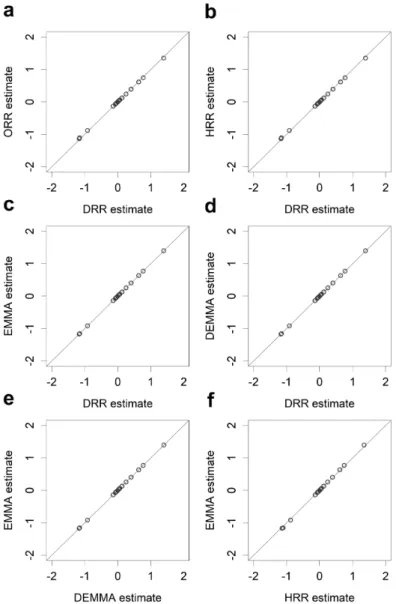
Figure 2.1 Pairwise comparisons of estimated effects from five different methods for the LASSO data. ... 40 Figure 2.2 Pairwise comparisons of the −log ( )₁₀ p test statistics from five different methods for the LASSO data. ... 41 Figure 2.3 Manhattan plots for KGW trait of the rice population consisting of 210

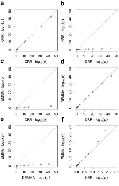
recombinant inbred lines from five different methods. ... 46 Figure 2.4 Pairwise comparisons of the −log ( )₁₀ p test statistics from five different methods for KGW of the rice population consisting of 210 recombinant inbred lines. ... 47 Figure 2.5 Manhattan plots for GW of the rice population consisting of 524 inbred varieties from five different methods. ... 49 Figure 2.6 Pairwise comparisons of the −log ( )₁₀ p test statistics from five different

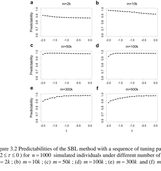
methods for GW of the rice population consisting of 524 inbred varieties. ... 50 Figure 3.1 Changes of estimated effects of 20 independent variables along with the change of the hyperparameter τ for the SBL method. ... 74 Figure 3.2 Predictabilities of the SBL method with a sequence of tuning parameter values (− ≤ ≤2 τ 0) for n=1000 simulated individuals under different number of markers. .... 75 Figure 3.3 Estimated effects of 1000 simulated markers on the first chromosome when the sample size is n=500 and the residual error variance is 2

10

σ = . ... 77

Figure 3.4 Statistical powers and Type 1 errors obtained at p=0.05 /m=2.5E−5 of four methods under four different experimental setups. ... 78

(13)

Figure 3.5 Statistical powers and FDR for four methods under four different experimental setups... 79 Figure 3.6 Statistical powers and Type 1 errors for four methods under four different experimental setups with threshold-A. ... 80 Figure 3.7 Statistical powers and Type 1 errors for four methods under four different experimental setups with threshold-B. ... 81 Figure 3.8 ROC curves of four methods under four experimental setups. ... 82 Figure 3.9 ROC curves (statistical powers plotted against Type 1 errors) drawn from 100 replicated simulations for SBL, BOLT-LMM and BSLMM when the number of causal SNPs is m_QTL =100. ... 87

Figure 3.10 ROC curves (statistical powers plotted against Type 1 errors) drawn from 100 replicated simulations for m=10k markers extracted from the hybrid rice genome. ... 88 Figure 3.11 Maximum memory usages for SBL, LASSO-A, LASSO-B, EMMA, BOLT-LMM and BSBOLT-LMM. ... 89 Figure 3.12 Test-statistic profiles of 1619 SNP bins in the RIL population of rice for KGW obtained from four methods. ... 92 Figure 3.13 Test-statistic profiles of 1619 SNP bins in the RIL population of rice for YD obtained from four methods. ... 93 Figure 3.14 Manhattan plots for GL of the hybrid rice varieties obtained from six

(14)

Figure 3.15 Manhattan plots for PN of the hybrid rice varieties obtained from six

methods... 99 Figure 3.16 Manhattan plots for PL of the hybrid rice varieties obtained from six

(15)

List of Tables

Table 2.1 Five GWAS methods under investigation and their Wald test statistics. ... 37 Table 2.2 The computational complexities of five GWAS methods. ... 38 Table 2.3 Estimated regression coefficients and variances of the estimates for 20

independent variables of the LASSO data obtained from five GWAS methods. ... 42 Table 3.1 Information of 20 simulated QTLs. ... 67 Table 3.2 Computing time of LASSO-B and SBL under 13 experimental setups with various sample size and number of markers. ... 83 Table 3.3 Statistical powers and FDRs of SBL, BOLT-LMM and BSLMM for the

simulation experiments with m=5, 10 and 50k markers extracted from the hybrid rice

genome when the number of causal QTLs is m_QTL =100. ... 86

Table 3.4 Statistical powers and FDRs of SBL, BOLT-LMM and BSLMM for the simulation experiments with m=10k markers extracted from the hybrid rice genome given three different numbers of causal QTLs (m_QTL =40,100,160). ... 86

Table 3.5 Significant QTLs identified by SBL, LASSO-B and EMMA for KGW of rice from the RIL population. ... 91 Table 3.6 Significant QTLs identified by SBL for YD trait of rice from the RIL

(16)

Chapter 1 Introduction

1.1 Quantitative trait locus mapping and genome-wide association studies

Most economically important traits in crops are quantitative in nature. Many disease susceptibility and behavior traits in human and animals are also quantitative in terms of their underlying genetic architectures. Loci controlling variation of these complex traits are called quantitative trait loci (QTL), which segregate and inherit following typical Mendelian laws of inheritance. However, QTL are not directly observable. DNA markers, also segregating according to Mendel’s laws of inheritance, can be observed. If an observed marker is associated with a quantitative trait, there must be QTL nearby the marker causing the observed marker-trait association. Detecting marker-trait association is called quantitative trait locus (QTL) mapping when the population is created through line crossing experiments (Soller 1978; Tanksley 1993; Doerge 2002) or genome-wide association studies (GWAS) if the population is a

randomly collected sample of a natural population (Hirschhorn and Daly 2005; Wang et al. 2005; Korte and Farlow 2013). Both QTL mapping and GWAS are essentially based on the principle of linkage disequilibrium that exists in the population under

investigation.

Mapping populations created through line crossing can be generally classified into biparental populations and multiparent populations depending on the number of parental lines. Common biparental populations for genetic analysis includes backcrosses (BC), F , ₂

(17)

double haploid (DH), recombinant inbred lines (RIL), near-isogenic lines (NIL), etc. The generation of biparental mapping populations is fast and easy to replicate, however, such populations only have limited recombination breakpoints and have limitations in the investigation on the dominant effects. To overcome the problems occurring in the

biparental populations, mapping population is constructed through multiparent lines such as nested association mapping (NAM), four-way (FW) cross, multiparent advanced generation intercrosses (MAGIC), etc.

With the phenotype and genotype data obtained from mapping populations, classical QTL mapping procedures detect association of trait with one locus at a time and the entire genome is then scanned with a finite number of discretized positions (loci) of the genome. If a locus does not overlap with a marker (such a locus is called a pseudo marker), the numerical codes of the genotypes are inferred from two markers flanking the locus, a technique called interval mapping (IM) (Soller et al. 1976; Lander and Botstein 1989; Haley and Knott 1992) because the two markers define an interval of the genome. Effects of QTL outside of the interval are captured by co-factors included in the model, a method called composite interval mapping (CIM) (Jansen 1993; Zeng 1993; Jansen and Stam 1994; Zeng 1994). The unique feature of IM or CIM is the inference of genotypes for pseudo markers bracketed by flanking markers. As the marker density becomes increasingly dense, the concept of interval no longer exists because it is redundant to infer genotypes of a pseudo marker whose genotypes are already observed. We are facing a challenge that is opposite to interval mapping – instead of inserting pseudo markers, we may need to skip markers because there are too many of them. With high marker

(18)

densities, the statistical technology used in GWAS has been adopted to QTL mapping. The co-factor selection step in composite interval mapping has been replaced by a polygenic effect modeled by a kinship matrix inferred from genome-wide markers (Xu 2013b).

GWAS represent a class of statistical methods for detection of genome-wide markers associated with quantitative traits (Schmid and Bennewitz 2017; Xu et al. 2017a; Wang et al. 2018). The idea of GWAS was initially proposed by Risch and Merikangas in 1996 stating that an association study on large scale genetic variants of unrelated

individuals is more powerful than a linkage analysis on a few hundred markers of individuals from an explicit pedigree, which pointed out the direction for the genetic studies of complex human diseases in the future (Risch and Merikangas 1996). However, the very first GWAS results were reported nearly ten years after and deemed as the real starting point of the GWAS era (Klein et al. 2005; DeWan et al. 2006; Consortium 2007). Since then, GWAS immensely attracted the attention of researchers from field of studies in human, animal and plant, and became a heated topic in quantitative genetics. In the next ten years, GWAS underwent a fast development with tens of remarkable statistical methods and more than 3,500 published papers (Buniello et al. 2018).

1.1.1 Linear mixed model

The population structure naturally forms accompanying subdivision of the original population. It universally exists among natural populations and may have

significant associations with genetic variants. Therefore, the population structure was the primary confounding factor of the early stage GWAS and the separation of true signals

(19)

from the false positive signals associated with population subdivision was necessary. Genomic control (GC) (Devlin and Roeder 1999) and structured association (SA) (Pritchard et al. 2000) are common methods to control the inflation of test statistics generated by population structure. GC algorithm assumes the population structure has equal effects on all loci, thus the overdispersion of the chi-squared test statistic is nearly the same across the entire genome (Devlin and Roeder 1999). The method was mainly applied to the case and control studies of human diseases and limited to biallelic markers. GC is based on a Bayesian probability model and uses a set of random marker to adjust the test statistics influenced by the population structure or cryptic relatedness among individuals. SA analysis uses random markers to infer the number of subpopulations and estimate the effect of population structure. It adopts a Bayesian clustering approach to calculate the probability of an individual being assigned to each subpopulation. Factors influencing the accuracy of the assignment to a subpopulation include the sample size, the number of markers, the amount of admixture, and the allele frequency divergence among subpopulations (Pritchard et al. 2000). The basic model of SA can be modified to handle correlated allele frequencies among different subpopulations and linkage

disequilibrium within subpopulations, which promotes its wide application in crop studies (Xu et al. 2017a).

With the development of GC, SA and other methods controlling the population structure, a unified mixed model method for association mapping that accounts for multiple levels of relatedness was proposed by Yu et al. in 2006 (Yu et al. 2006). This most commonly used method is also called the Q+K linear mixed model (LMM)

(20)

approach (Q represents the population structure and K represents the kinship matrix among individuals inferred from genome-wide markers), which is a powerful tool for both QTL mapping and GWAS as they share the same theoretical basis. The mixed model equation for the Q+K method is

y= Xβ+Sα +Qv+Zu+e (1.1) where β is a vector of all fixed effects except the effects of marker and population structure, α is a vector of SNP (or marker) effects, v is a vector of population effects, u is a vector of polygenic effects, e is a vector of residual errors, X S, and Z are design matrices. The population structure matrix Q can be obtained by GC and SA. The authors implemented the model by using the mixed procedure in SAS (PROC MIXED) to scan the genome for signals of marker trait association.

The original LMM approach has two major contributions to association studies. First, it detects genetic variants with simultaneously controlling the multiple level cryptic relatedness among individuals. Second, it promotes the use of marker inferred kinship matrix, which overcomes the limitations of association studies in the population lack of complete pedigree records. Besides, another benefit of LMM is the flexibility to drop either Q or K from the model to adapt the population under testing. Q can be dropped if population structure does not exist and the model is reduced to a single population-based association study with correction of polygenic effects. K is safely dropped when

individuals within each subpopulation are random mating and the model turns into a regression-based structured association analysis (Yu et al. 2006). Many investigations showed that the model with the inclusion of Q+K leads to more accurate estimation of

(21)

marker effects than the model only involving one correction matrix (Xu et al. 2017a; Wang and Xu 2019).

1.2 Single locus model based GWAS

1.2.1 Development of single locus model based GWAS

The computational speed of the mixed model was a great challenge to the original LMM analysis. Following the first Q+K LMM, a large number of approximate and improved methods were published in a span of about decade years. Now, methodology development has been cooling down. Typical examples include, but not limited to, the following significant modifications.

Principal components analysis (PCA)(Price et al. 2006) summarizes the genome-wide patterns of relatedness among individuals by several components without requiring the explicit classification of subpopulations. Zhao et al. (2007) suggested that the Q matrix in the original LMM can be replaced by principal components (PCs) to avoid intensive computation of population structure. In their association mapping of an Arabidopsis F2 population, both GC and PCA capture the underlying structure reasonably well, however, PCA is more efficient in terms of computation time.

In the same year, a genome-wide rapid association using mixed model and regression (GRAMMAR) was developed by Aulchenko et al. (2007). In this method, a polygenic random effect was fitted to a null mixed model without marker effect to estimate residual errors, and then the residual after fitting the polygene was treated as a new response variable for GWAS by testing one marker at a time with a simple linear regression analysis. Therefore, the computation time of GRAMMAR for each SNP is

(22)

reduced to be linear with the number of individuals included in the model. This method is an approximation of the LMM and is no longer used after more advanced methods have been published.

The next milestone improvement is the efficient mixed model association

(EMMA) by (Kang et al. 2008). The authors first performed eigenvalue decomposition of the kinship matrix and then transformed the response variable and the design matrix of the fixed effects (including the Q matrix and the current marker under investigation) by the eigenvector (a matrix) so that repeated inverse of a large kinship matrix has been avoided. This is an exact method with no compromise in statistical power and Type 1 error control. Kang et al. (2010) also simplified the original EMMA method by fixing the estimated genomic heritability of trait at the null model and then scanned the genome under the given heritability value. This method is called efficient mixed-model

association eXpedited (EMMAX) (Kang et al. 2010). A similar approximation approach proposed by Zhang et al. (2010) is called “population parameters previously determined” (P3D). P3D estimates variance components from the null model and fixes these

parameters when testing each SNP marker, thus, variance components do not need to be estimated repeatedly. At that moment, it appeared that the limiting factor was no longer the number of markers but the sample size (n) because eigenvalue decomposition is performed on the kinship matrix with a time complexity of 3

( ) O n .

The next improvement focused on computational speed and the method is called the factored spectrally transformed linear mixed models (FaST-LMM) (Lippert et al. 2011). They reduced the number of markers used to calculate the kinship matrix into a set

(23)

smaller than the sample size but still capture the main feature of the kinship matrix. When the selected number of markers (m₀) is smaller than the sample size (n), the time

complexity of decomposition of the kinship matrix becomes O m( 3₀). When the number of

markers is small, the competition between the marker under test and the same marker in the kinship matrix cannot be ignored. Therefore, they used the same spectrally

transformed method to decompose the kinship matrix again to adjust the kinship matrix to reduce the competition (Lippert et al. 2011). This method (FaST-LMM) is currently the most efficient method for GWAS in large populations.

The genome efficient mixed model association (GEMMA) developed by Zhou and Stephens (2012) is nearly the same as the original EMMA (Kang et al. 2008) but incorporating an efficient recurrent algorithm to transform the data and a combination of grid search and Newton’s method to find the solution of the polygenic variance

component. This new method is approximately n times faster than EMMA, where n is the number of individuals. GEMMA is an exact method that the variance components are re-estimated for each marker and provides the exactly same Wald or likelihood-ratio test statistics as EMMA.

Loh et al. (2015) bridged the frequentist association testing and the Bayesian modeling, and developed a new method called efficient Bayesian mixed-model

association (BOLT-LMM). Comparing to all existing methods implementing the linear mixed models at that time, BOLT-LMM requires only O mn( ) iterations to analyze genome-wide markers, which is at least n times faster than the previous methods. A detailed discussion of BOLT-LMM will be provided later.

(24)

1.2.2 Ridge regression

Ridge regression was first proposed as a regularized regression method by (Hoerl 1962) and formalized by Hoerl and Kennard (1970). The method was designed to handle highly correlated independent variables (collinearity problem). When multi-collinearity occurs, the inverse of the coefficient matrix (X XT ) is not stable, leading to large standard errors of the estimated coefficients. Adding a small positive number to the diagonal of matrix X XT will introduce a small bias to the estimates but can substantially reduce the estimation errors. When the number of independent variables is large, multi-collinearity can also occur, even if the pair-wise correlations of the independent variables are mild. Therefore, ridge regression has been used for prediction when the number of independent variables is larger than the sample size (Hastie et al. 2001; Hastie and Tibshirani 2004).

In the genome era, ridge regression has been substantially used for genomic selection (Piepho 2009; Endelman 2011). Because the independent variables are numerically coded genotypes of genome-wide markers, ridge regression is also called genomic best linear unbiased prediction (gBLUP). Compared with other statistical methods of genomic selection, gBLUP is often the best method in terms of high

predictability and fast computational efficiency (Lorenzana and Bernardo 2009; Xu et al. 2014; Xu et al. 2016; Xu et al. 2017b). However, gBLUP has not been routinely used for GWAS because the test statistics are often too low due to shrinkage of the estimated regression coefficients. Malo et al. (2008) used ridge regression to detect marker trait

(25)

association aiming to simultaneously detect multiple linked markers. Since the number of markers was relatively small in their analysis, the test statistics were not shrunken too much and their results were acceptable. Shen et al. (2013) proposed a generalize ridge regression for GWAS, in which a conventional ridge regression (rrBLUP) was performed with the shrinkage parameter 2 2

ˆe / ˆb

λ σ σ= estimated from the maximum likelihood

method and then followed by a second step to retune the coefficients under

heterogeneous shrinkages. The heterogeneous shrinkages are represented by ˆ2/ ˆ2

k k e b λ =σ σ where ˆ2 k b

σ depends on the ridge coefficients obtained from the conventional ridge

regression. The second step is not iterative and thus can be very fast. The retuned coefficients are very close to the coefficients estimated from Bayes A (Meuwissen et al. 2001) but obtained with a speed magnitude faster than Bayes A. Duarte et al. (2014) recognized the over shrinkage of ridge coefficients and their test statistics, and proposed to adjust the test statistics to a level similar to the tests from the conventional GWAS under LMM. They replaced the error variances of estimated coefficients by variances derived by Henderson (1975). When the marker density is high, Henderson’s variance is often smaller than the error variance, leading to a higher test statistic. Real data analysis and simulation studies (Duarte et al. 2014) showed that the adjusted tests are very close to the tests obtained from the EMMA study. To take advantage of the computational

efficiency of this adjusted method, Ning et al. (2018) extended the method to detect epistatic effects (gene by gene interactions), while detection of all pair-wise epistatic effects was impossible for any conventional GWAS methods if the marker density is larger than, say, ten thousands.

(26)

1.2.3 Significance test

Single locus model-based GWAS approaches detect association of trait with one SNP at a time and the analysis will be finished until the entire genome is scanned. In fact,

m independent tests are performed in the analysis, where m is the number of markers. Therefore, the nominal probability p=0.05 should not be used intuitively in significance testing, and a correction of multiple tests is required. Bonferroni correction is the simplest and most conservative way to correct multiple tests. It adjusts the original critical value by dividing the number of tests involved (from p=0.05 to p=0.05 /m). A less stringent approach proposed by Benjamini and Hochberg (1995) is controlling the false discovery rate (FDR) or the expected proportion of falsely rejected hypotheses. Suppose

1, ,2 , m

P P  P are p-values of multiple statistical tests H₁, ,H₂ ,Hm. These p-values are firstly ordered in an ascending order that P₍₁₎≤P₍₂₎≤≤P_{( )}_m . Then let k be the largest i for which P_{( )}_i ≤( /i m q) * and reject all H i_{( )}_i =1, 2,,k (q* is the nominal level of FDR, say 0.05)(Benjamini and Hochberg 1995). An alternative method without specifying the pre-determined threshold is permutation (Churchill and Doerge 1994), which is

commonly practiced in real world data-based GWAS. In permutation, observations of a trait are shuffled to disrupt the original sequence and generate a new vector of

observations, which breaks the underlying association between genotype and the real phenotype. This shuffle procedure must be repeated for many times (usually ≥1000) and the same association analysis is performed on each of these permutation experiments. Test statistics from large scale permutations form the null distribution for researcher to

(27)

select empirical threshold used in significance test. This approach has benefit in providing reliable results but is not computationally efficient.

Besides the three common practices mentioned above, one can replace the total number of tests by the effective number of tests in multiple testing correction (Moskvina and Schmidt 2008). Effective number of tests is inferred from the linkage relationship of the genotype and greatly reduces the actual number of tests. Mackay (1992) proposed a similar concept under Bayesian framework, the effective number of well-measured parameters (marker effects) determined by the data. Tipping (2001) interpreted it as a measure of how “well-determined” a random effect is by the data. The degree of

confidence for each marker effect is the complement of the ratio of the posterior variance to the prior variance. The total effective number of markers (the same as effective

number of tests) equals the sum of all confidences. This concept attracts much attention and gains potential applications not limited to multiple testing correction (Xu 2013a; Wang et al. 2016).

1.3 Multiple locus model based GWAS

1.3.1 Development of multiple locus model based GWAS

Both QTL mapping and GWAS are based on the linkage disequilibrium (LD) that naturally existing in the genome. LD is the non-random association of alleles at different loci in a general population (Slatkin 2008) and created by recombination, non-random mating, and evolutionary force factors including selection, mutation, migration and genetic drift. On the other hand, it can be broken down by recombination events (Hartl and Clark 1997). Stronger LD indicates a smaller genetic distance is often observed

(28)

among loci that are physically close together than among loci that are farther apart on a chromosome (Hill and Robertson 1968). One common feature of the single locus mixed model QTL mapping and GWAS is that both detect association of trait with one locus at a time until all loci are detected to complete the analysis. Technically, such single locus model is one-dimensional scanning approach. As a result, one often expects to see an island surrounding a high peak in a Manhattan plot, which is caused by LD. This island behavior of the Manhattan plot will drastically change if all markers are included in the same statistical model with effects being estimated simultaneously. The multiple locus model often eliminates the island, leaving a single peak standing alone. This single peak is supposed to be better than an island because the signal is cleaner and stronger, but most people do not trust the single peak.

Multiple QTL linkage studies were invented two decades ago (Green 1995; Jiang and Zeng 1995; Nakamichi et al. 2001; Sen and Churchill 2001) represented by the multiple interval mapping of Kao et al. (1999), which was carried out via step-wide variable selection. The method is computationally intensive and thus rarely used by the QTL mapping community. Multiple locus GWAS is also available and mainly conducted via Markov chain Monte Carlo (MCMC), a technique also very intensive

computationally. Current multiple marker models that have been applied to QTL mapping and GWAS include the least absolute shrinkage selection operator (LASSO) (Tibshirani 1996), empirical Bayes (Xu 2007), multi-locus mixed model (MLMM) (Segura et al. 2012) and Bayesian sparse linear mixed model (BSLMM) (Zhou et al. 2013). With the exception of LASSO, the other three methods are slow in terms of

(29)

computational speed. LASSO is surprisingly fast for small and intermediate sample sizes (from approximately 200 to 5000) but can fail for large samples with extremely high marker densities.

Modified from the ordinary least square (OLS) regression, LASSO minimizes a loss function composed of the residual sum of squares and the sum of the absolute values of coefficients. The special constraint produces some coefficients equal to zero and shrinks the rest of coefficients for easier interpretation than OLS and ridge regression (Tibshirani 1996). LASSO is widely used in variable selection because of its strong shrinkage on regression coefficients. Park and Casella (2008) assigned an independent double-exponential prior to each coefficient and interpreted the LASSO with Bayes theorem (Bayesian LASSO). Yi and Xu (2008) improved the application of Bayesian LASSO procedure in QTL mapping by modifying prior distributions for the variances and the estimation of hyperparameter. Another improvement on LASSO is the liner mixed model-LASSO (LMM-Lasso), which detects multiple causal loci simultaneously with the correction of confounding effects, such as population structure (Rakitsch et al. 2013).

Empirical Bayes (E-BAYES) method developed by Xu (2007) is a Bayesian method by assigning each marker effect a normal prior distribution and the prior variance is estimated from the data. It provides optimal estimation of variance components and makes selective shrinkage on marker effects that large effects virtually receive no shrinkage while small effects are penalized to zero. The author estimates variance components by maximizing the logarithmic likelihood function instead of MCMC

(30)

sampling steps. The optimization involves a special multiple step algorithm that updates one variance component at a time conditional on all other variance components. Even if the method does not involve MCMC sampling steps, the implementation of E-BAYES is somewhat time consuming.

Segura et al. (2012) proposed the multi-locus mixed-model (MLMM) to detect causal genetic variants on a genome-wide basis with the control of confounding caused by population structure. MLMM can handle the problem of mn and uses a stepwise algorithm of forward inclusion and backward elimination to speed up the regression. In the forward inclusion step, the most significant marker is added to the model as a

cofactor, then p-values for all cofactors and variance components are re-estimated for the next inclusion step. The forward step stops when the heritable variance estimate is close to zero and the backward elimination starts to repeatedly drop the least significant cofactor in the model.

The hybrid method of LMM and sparse regression model (BSLMM) presented by Zhou et al. (2013) can perform model fitting and prediction simultaneously in a single analysis. They specify appropriate prior for the hyperparameters and use a new MCMC approach for posterior inference. We will discuss this method in detail in the section 1.4.4.

1.3.2 Optimization by coordinate descent

The data used in GWAS tends to include large sample size with a large number of SNP markers because the DNA sequencing cost is cheap and not a financial concern anymore. However, large m and n cause a problem that the model space becomes too

(31)

large to explore (Segura et al. 2012). Therefore, the investigation of the single locus model for GWAS is earlier and more thorough than that of the multi locus model. A challenging problem of the association studies using multi locus model is that the number of observations can be much less than the number of markers in a GWAS dataset (mn ), which is also known as the “large p small n” problem in statistical modeling that the sample size is substantially smaller than the number of available covariates (Chakraborty et al. 2012), and the problem is more complicated when markers are highly correlated.

Coordinate descent (CD) algorithm is an iterative method that updates one regression coefficient at a time. Within each iterative step, the model minimizes the objective coefficient with fixing the rest coefficients of the variable vector at the values estimated from the previous iteration. Therefore, the entire complicated problem is decomposed into many low-dimensional subproblem, which substantially can be solved easily than the original model fitting (Wright 2015). CD is commonly used in high dimensional data analysis and becomes an important tool of optimization in the “big data” era. According to Wright (2015), in a linear system Aw=b, the least-norm

solution is min(1 2 w 2₂). By setting w=A xT , the corresponding Lagrangian dual is

2 2

min ( )f x =1 2 A xT −b xT . The k-th iterative step has the form of

1

( )

k k T k

ik ik ik

x + ←x − A A x −b e , where i denotes the i-th row of the matrix for i=1, 2,,n and e_ik is the residual. The solution of the original linear problem wk is estimated by the

update of k x , 1 ( ) ( ) k k T k T k k T ik ik ik ik ik ik w + ←w − A A x −b A =w − A w −b A (1.2)

(32)

and the i_k equation of Aw=b is satisfied by 1 ( ) k k k ik ik ik ik ik A w + =A w − A w −b =b (1.3)

Coordinate descent is commonly used in minimizing the ridge and LASSO loss functions (Hastie et al. 2001). In addition, the basic CD has been modified to solve a wide variety of problems such as block CD for sparse inverse covariance estimation (Friedman et al. 2008), cyclic CD approach for determining protein structure (Canutescu and Dunbrack Jr 2003), etc.

1.4 Common GWAS methods 1.4.1 EMMA

Kang et al. (2008) found three major limitations of the original form of LMM method. First, the variance components estimation algorithm involved in the original LMM method only provide local solution, which leads to inaccurate statistical inferences. Second, the optimization procedure requires extensive matrix calculation within each iteration, thus the computation is even more expensive for the entire analysis. Third, the kinship matrix involved in LMM method is not guaranteed to be positive semidefinite, which may not be a correct form of variance component. To conquer these problems, Kang et al. (2008) proposed the EMMA to describe the association of observed phenotypes as

y= Xβ+Zu+e (1.4)

where y is an n×1 vector of phenotypic values, X is an n q× design matrix for all fixed effects, β is a q×1 vector of fixed effects, Z is a n t× matrix of genotype indicator

(33)

2 ~ (0, )

u N σ K , and e is an n n× matrix of residuals that 2 ~ (0, e )

e N σ I . K is the t t× kinship matrix measuring the relatedness between every pair of individuals. The variance-covariance matrix of phenotypes is

2 2

var( )y = =V σ ZKZT +σ_eI (1.5)

The log-likelihood function of the full model is

2 1 2 1 1 ( ; , , ) log(2 ) log | | ( ) ( ) 2 T F l y β σ δ n πσ H y Xβ H y Xβ σ −   = _− − − − − _   (1.6)

and restricted log-likelihood function is

2 1 2 1

ˆ

( ; , ) ( ; , , ) log(2 ) log | | log | |

2 T T R F l yσ δ =l y β σ δ + _q πσ + X X − X H X− _ (1.7) where H =V σ =ZKZT +δI and 2 2 e

δ σ σ= . Kang et al. (2008) used spectral

decomposition to ease the computational load,

1

diag( , , ) T

F n F

H =U ξ δ+  ξ +δ U (1.8)

where U_F is an n n× matrix of eigenvectors and diag(ξ δ₁+ ,,ξ δ_n+ ) is holding the eigenvalues. The maximization of full model likelihood function and restricted likelihood function turns into the optimization of functions with respect to δ , because δ is the only parameter involved in the likelihood function. The estimation of variance components

2 2

and _e

σ σ is simplified to the optimization of δ for each marker. The computational

complexity of the method implementing eigen decomposition is O n( 3+rn), in contrast, the standard expectation-maximization and Newton-Raphson algorithms require the computational complexity of O rn( 3), where r is the number of iterations required by

(34)

optimization. EMMA performs eigen decomposition only once while previous methods require matrix multiplications and inverses for each iteration (Kang et al. 2008).

EMMA is a milestone in the development of single locus model-based GWAS methodology. It increases the computational efficiency of the original LMM method and effectively control the inflated false positives caused by genetic relatedness. EMMA calculates global solution of likelihood function and the convergence with a smaller search space is guaranteed. Since it was published, many modifications had been

proposed to lower the computational cost and many impactive methods are derived from it (Kang et al. 2010; Zhang et al. 2010; Zhou and Stephens 2012).

1.4.2 BOLT-LMM

BOLT-LMM, proposed by Loh et al. (2015) made two breakthrough compared with the conventional single locus GWAS methods. Before the invention of BOLT-LMM, other existing methods require computational complexity of O mn( 2) or O m n( 2 ). In contrast, BOLT-LMM only requires time cost O mn( ), which is at least ntimes less than previous methods (in most cases, m>n). The algorithm is built on the theoretical basis of non-infinitesimal genetic architectures and fits a mixture of two Gaussian distributions of marker effects to increase statistical power. The authors believed that the assumption of an infinitesimal genetic architecture and the normal distribution of effect sizes limit the power of existing methods. The BOLT-LMM involves four major steps: (1) Estimation of variance components by using a stochastic approximation algorithm. The estimates are nearly identical to those estimated by standard approach, but the time and memory costs are reduced.

(35)

(2) Calculation of association statistics based on the infinitesimal mixed-model. This step is accomplished via the conjugate gradient iterations to avoid spectral decomposition of the kinship matrix.

(3) Estimation of parameters involved in Gaussian mixture model. BOLT-LMM uses a mixture of two Gaussian distribution as the prior for marker effect sizes to capture both the large effects and small genome-wide effects.

(4) Calculation of Gaussian mixture model association statistics. In this step, each marker is tested against the residual phenotype obtained from the model involving Gaussian mixture distributions. Association statistics obtained from step (2) are calibrated by LD Score regression (Bulik-Sullivan et al. 2015).

The algorithm is built upon Bayes’ theorem and uses a variational approximation to compute approximate phenotypic residuals rather than MCMC as in many Bayesian methods. The hyperparameters involved in the variational approximation is estimated by cross-validation instead of maximizing the log-likelihood function. Marker is tested for association with the residuals by a retrospective score statistic. The association evidence of each marker is given in the form of p-value whereas other popular Bayesian

approaches provide the posterior inclusion probability as the evidence of association. The method links the frequentist association testing and the Bayesian modeling together for phenotypic prediction.

1.4.3 LASSO

LASSO is widely used and testified to be very useful in feature selection and genomic selection (GS)(Usai et al. 2009; Li and Sillanpää 2012; Xu et al. 2016).

(36)

However, the method has never been commonly used for GWAS because the glmnet/R package (Friedman et al. 2010) implementing the LASSO method does not provide a mechanism to calculate the standard errors of estimated effects and thus cannot perform statistical tests for markers. Lockhart et al. (2014) then proposed the covariance test statistic based on lasso fitted values to test the significance of predictor variables. However, the method is suitable for the dataset of which the number of markers is less than the sample size. To better accommodate high-dimensional case mn, Ithnin et al. (2017) recently developed two methods to calculate the standard error of each estimated marker effect which allows the further calculation of Wald test statistic for significance test. One method uses bootstrap approach (Efron and Tibshirani 1994) where a large number of bootstrap samples (say 1,000) are drawn and analyzed by glmnet/R to obtain the empirical standard error of each estimate, and the other method is based on the BLUP equation (Henderson 1975).

They define ˆβj for j=1,,S as effect estimates of markers selected by LASSO (S <m). The Henderson mixed model equation for these effect estimates is

1 0 0 0 1₂ ₂ 0 0 0 1 0 1 1 1 1 1 2 2 0 1 ˆ ˆ / ˆ / S T T T _T S T T T _T S T T T T S S S S S S X X X X X X _{X y} X X X X X X _{X y} X y X X X X X X β β β σ σ _β σ σ _β  _{   }   + _{   }₌   _{   } _  ₊ _{   } _    _{ }              (1.9)

where y is an n×1 vector of phenotypic values of the trait under study, X₀ is an n×1

vector of unity, X_j (for j=1,,S) is an n×1 vector of genotype indicator variables for the selected marker j, β₀ is the interceptor grand mean, and σ2 is the residual variance.

(37)

The prior variance of each marker effect is 2

j β

σ , which is the unknown of the BLUP

equation. Ithnin et al. (2017) replaced 2

j β

σ by βˆ2_j to obtain the approximate

variance-covariance matrix of coefficient estimates

1 0 0 0 1 0 0 2 2 2 1 0 1 1 1 1 1 2 2 0 1 ˆ ˆ ˆ _/ ˆ var ˆ ˆ _/ T T T S T T T S T T T S S S S S S X X X X X X X X X X X X X X X X X X β σ β β _σ σ β β −        ₊  =         +               (1.10)

where σˆ2 is the estimated residual variance. Compared to the bootstrap approach, this approximation is much more efficient in terms of computing time. Simulation studies indicate that the LASSO with bootstrapped standard error calculation has perfect power for detecting true QTLs, followed by LASSO with BLUP error calculation. Both multiple locus methods outperform the popular single locus model based method GEMMA (Ithnin et al. 2017).

1.4.4 BSLMM

Both LMM and sparse regression model are commonly applied to polygenic modeling in association studies. Compared to single marker test of association, polygenic modeling relates phenotypic variation to many genetic variants simultaneously. It should be noticed that the assumptions on the genetic structure of a population behind these two models are different. In polygenic modeling, the LMM assumes that the phenotype is affected by every genetic variant and the effect of each marker is normally distributed. In contrast, sparse regression model assumes that among all genetic variants, only a small proportion of them have effects on the phenotype. To merge the two assumptions together, Zhou et al. (2013) developed a hybrid to include both models called BSLMM.

(38)

Benefit from two widely used models, the BSLMM method can perform GWAS, variance components estimation and phenotype prediction simultaneously.

The BSLMM method adopts a standard linear mixed model

1_n

y= µ+Xβ+ +u ε (1.11) where y is an n×1 vector of phenotypes measured on n individuals, 1_n is an n×1

vector of 1s, µ is the mean of phenotypes, X is an n×p matrix of genotype indicator

variables measured on n individuals at p genetic markers, β is a p×1 vector of unknown genetic marker effects referred as “sparse effects” to emphasize the sparsity-inducing prior, u is an n×1 vector of random effects, and ε is an n×1 vector of residual error terms. The effect of every marker comes from a mixture of two normal distributions

2 1 0 ~ (0, ) (1 ) i N a β π σ τ− _{+ −}π δ (1.12)

where π is the proportion of non-zero β and δ₀ denotes a point mass at zero. , , , and _a

µ τ π σ are the hyperparameters. Random effects are obtained from their

posterior distribution given the observed data via Markov chain Monte Carlo (MCMC). In the association test, BSLMM does not provide the p-value of a marker for significance test, instead, it summarizes a posterior inclusion probability (PIP) of every marker. The posterior inclusion probability is the probability that the marker has a sparse effect and associate with the trait given the data. Lloyd-Jones et al. (2017) implemented BSLMM in association studies of human eye and skin color. Because BSLMM analyzes all loci simultaneously, markers in high LD maybe jointly detected to affect the trait other than attribute the signal to a specific marker. Therefore, the best way to infer the marker’s

(39)

significance from BSLMM is based on genomic windows instead of individual SNPs (Lloyd-Jones et al. 2017). Guan and Stephens (2011) suggested that the posterior expected number of SNP markers within a window can be obtained by summing up the PIPs of all markers in that window, named WPIP. One can compare the WPIP

(40)

Chapter 2 Deshrinking ridge regression for linkage analyses and

association studies

2.1 Introduction

In the big data era, QTL mapping and GWAS are further challenged by the presence of multiple omic data, e.g, transcriptome, metabolome, phenome, epigenome and so on. These omic data can be treated as predictors like genome (Xu et al. 2016; Xu et al. 2017b) to predict agronomic traits, but they are more often considered as response variables (Gong et al. 2013; Wang et al. 2014; Wen et al. 2014). For example, expression of a transcript can be treated as a quantitative trait and QTL mapping is performed on this expression trait. Such a QTL mapping is called expression trait QTL mapping, i.e., eQTL mapping (Wang et al. 2014; Wen et al. 2014). A microarray experiment can

simultaneously generate more than 20 thousand expression traits. Mapping QTL for that many traits requires more efficient statistical methods with speed many times faster than even the fastest method currently available. All the single locus models are based on a genome scanning scheme and further improvement can only be achieved via parallel computing. In this study, we propose a ridge regression for QTL mapping and GWAS and hope to improve the computational efficiency to a different level.

In this study, we re-evaluated the method of Duarte et al. (2014) and proposed a new adjustment with more rigorous theoretical support. The new method is called

(41)

high) while the method of Duarte et al. (2014) performs poorly when the marker density is very low. We compared the computational efficiencies of the new method with EMMA and several other methods on three datasets with different model sizes (small, medium and large). We show that DRR is efficient for all model sizes while EMMA is only useful for medium and large models.

2.2 Materials and methods 2.2.1 Data used for illustration 2.2.1.1 The LASSO data

This dataset is the “QuickStartExample” data downloaded from the R package “glmnet” (Friedman et al. 2010). The dataset contains 100 observations for 20

independent variables (x) and one response variable (y). Below is the R code to load the data,

library(glmnet)

data(QuickStartExample)

The dataset was analyzed using all methods described in the Methods section, including ORR, HRR, DRR, EMMA and DEMMA. The purpose of this data analysis is to

investigate the properties of all methods for small models.

2.2.1.2 The rice QTL mapping data

The second data contains 1619 markers (independent variables) from 210 recombinant inbred lines of rice (Yu et al. 2011). Average of the thousand grain weight (KGW) trait measured from four replicates is the response variable. The purpose of this data analysis is to evaluate the properties of all methods for intermediate models.

(42)

2.2.1.3 The rice GWAS data

The GWAS data consist of 524 inbred varieties of rice collected from China and southeast Asia (Chen et al. 2014; Wei et al. 2018). The trait analyzed is the grain width, a highly heritable trait. After the imputation and quality control, 6.5 million SNPs covering about 90% of total SNPs in rice were published by Chen et al. (2014) on the RiceVarMap website (http://ricevarmap.ncpgr.cn/v2). Among 6.5 million SNPs, we randomly selected 310,000 SNPs for further analysis. By using this data, we investigated the properties of the five methods when applied to large models.

2.2.2 Ordinary ridge regression (ORR)

Deshrinking ridge regression (DRR) for GWAS is a method to correct the bias of a ridge estimated regression coefficient (marker effect) so that it is comparable to the estimated marker effect from the efficient mixed model association (EMMA) study in which a marker is treated as a fixed effect. The new DRR method for GWAS is computationally more efficient then EMMA. In this section, we will review the basic concept of ordinary ridge regression (ORR) before introducing DRR. The EMMA procedure and a decontaminated efficient mixed model association (DEMMA) method will be compared with the new method.

The ordinary ridge regression is equivalent to the best linear unbiased prediction (BLUP). Let y be an n×1 vector of phenotypic values for a quantitative trait. Define Z as an n m× matrix for the genotype indicator variables of m markers. Let X be an n q× design matrix for some systematic (fixed) effects unrelated to genetics. The linear model for y is

(43)

y= Xβ+Zγ ε+ (2.1) where β is a q×1 vector of fixed effects, γ is an m×1 vector for the effects of all m markers and ε is an n×1 vector of residual errors. Each marker effect is assumed to be normally distributed with a common variance, i.e., 2

~ (0, ) k N

γ φ for all k=1,,m. Each residual error is also assumed to be normally distributed, i.e., ε_j ~ N(0,σ2) for all

1, ,

j=  n. The expectation and variance of y are E( )y = Xβ and

2 2 2 2 2 2

var( )y =ZZTφ +Iσ =Kφ +Iσ =(Kλ+I)σ =Hσ

respectively, where K =ZZT is a marker inferred kinship matrix, λ φ σ= 2 / 2 and H =Kλ+I. The restricted maximum likelihood (REML) method is used to estimate parameters. Eigenvalue decomposition of the kinship matrix, T

K =UDU , is incorporated into the likelihood function to improve computational efficiency (Kang et al. 2008; Zhou and Stephens 2012). Given the REML estimates of the variance parameters, we can immediately write the BLUP of all marker effects and their variances using the conditional expectation and conditional variance shown below,

1 1 ˆORR E( | )y ZT(K I) (y X ) Z HT (y X ) γ ₌ γ ₌λ λ₊ − ₋ β ₌λ − ₋ β (2.2) and 2 2 2 2 1 2 1 2 var(γORR| )y =φ I−φ ZT(Kφ +Iσ )− Zφ =(λI−λZ H ZT − λ σ) (2.3) Note that 1 1 ( ) T

H− =U Dλ+I −U and computation of the inverse is very cheap because Dλ+I is a diagonal matrix. For marker k, the BLUP and its variance are simply the kth element of ˆγORR and the kth diagonal element of var(γˆORR | )y , i.e.,

(44)

1 ˆ_kORR Z H_kT (y X ) γ ₌λ − ₋ β (2.4) and 1 2 ˆ var( ORR| ) ( T ) k y Z H Zk k γ ₌ λ λ₋ − λ σ (2.5)

The Wald test for this ordinary ridge regression (ORR) is defined as 2 ORR (ˆ ) ˆ var( | ) ORR k k ORR k W y γ γ = (2.6)

Under the null model H₀:γ =_k 0, W_kORR does not follow a Chi-square distribution

because ˆORR k

γ is a shrinkage estimate. This explains why ridge regression has not been

used as a tool for GWAS.

2.2.3 Wald test using Henderson’s variance (HRR)

Using Henderson’s (1975) notation, the variance for the BLUP of a random effect is var(γˆ_kORR−γ_k)=var(γˆ_kORR| )y . Henderson provided another variance for the BLUP,

2 1 2 1 2

ˆ ˆ

var(γ_kORR)=var(γ_k)−var(γ_kORR| )y =λσ −(λ λ− Z H Z_kT − _kλ σ) =λZ H Z_kT − _kλσ (2.7)

where 2 2

var(γk)=φ =λσ . Duarte et al. (2014) realized that when the number of markers

is large, this variance is much smaller than var(γˆkORR| )y and thus a Wald test using this

smaller variance will boost the test statistic. Therefore, they proposed the following Wald test and we call this test Henderson’s ridge regression (HRR),

2 2 2 HRR 1 2 ˆ ˆ ˆ ( ) ( ) ( ) ˆ ˆ

var( ) var( ) var( | )

ORR ORR ORR

k k k k ORR ORR T k k k k k W y Z H Z γ γ γ γ γ γ λ − λσ = = = − (2.8)

Duarte et al. (2014) compared W_kHRR with W_kEMMA (Wald test from EMMA) and observed

(45)

recommended using Henderson’s Wald test in place of W_kEMMA to improve computational

efficiency for GWAS.

2.2.4 Deshrinking ridge regression (DRR)

Henderson’s Wald test proposed by Duarte et al. (2014) has brought the shrunk test statistic back to the level comparable to the test of the conventional GWAS such as EMMA method (Kang et al. 2008) and GEMMA method (Zhou and Stephens 2012). However, the authors did not address how to bring the estimated effects back to the same levels as the conventional GWAS. In addition, when the number of markers is small, say less than 1000, Henderson’s variance may be greater than the variance of prediction and thus may lead to a reduced test statistic. Although m≤1000 is very rare in GWAS, a statistically rigorous test should apply to all genome sizes. Therefore, we propose the following deshrinking ridge regression (DRR) that can bring both the effects and the tests back to the levels comparable to the conventional GWAS.

We first introduce the “well-measurement-factor” (also called degree of freedom) for a predicted random marker effect and use it to deshrink the random effect up to the level comparable to the estimate as if it were estimated from a fixed effect model. The concept of “degree of freedom” was proposed by (Mackay 1992). He used the estimated mean of a variable as an example to demonstrate the concept. The estimated mean used to calculate a sample variance is a well measured parameter (fixed effect). It counts for one degree of freedom and thus the sum of squares must be divided by n – 1 to give an unbiased estimate of the variance. If an effect is treated as random, then it is not well measured. The degree of freedom of the random effect is derived from the Bayes

(46)

theorem. When γ_k (effect of marker k) is treated as a random effect, its prior distribution

is N(0,φ2). The posterior distribution is N(γˆ_kORR,Vˆ_kORR), where ˆORR k

γ is the shrunk

estimate from the ORR and ˆV_kORR =var(γˆ_kORR | )y =var(γˆ_kORR−γ_k) is the variance of prediction. The corresponding deshrunk estimate and deshrunk variance of marker k are denoted by ˆDRR

k

γ and ˆV_kDRR =var(γˆ_kDRR), respectively. They are the fixed effect equivalent

counterparts and are the quantities we need to perform Wald test for association studies. The new method is based on Mackay’s (1992) well-measurement-factor for a predicted random effect. The factor is

1 2 1 2 ˆ var( | ) ( ) 1 1 var( ) ORR T T k k k k k k k y Z H Z d γ λ λ λ σ λZ H Z γ φ − − − = − = − = (2.9) where 2

var(γ_k)=φ and var(γ_k | )y are interpreted as the prior and posterior variances,

respectively, for the random effect. If it were a fixed effect, the prior variance would be infinity and thus d_k =1, the parameter being well determined. For a random effect, unless

the posterior variance is closed to 0 (occurs when the sample size is infinity), the degree of freedom is between 0 and 1.

It is well known that the posterior mean and posterior variance of γ_k can be expressed as 1 1 2 2 2 ˆ 1 1 0 1 1 ˆ ˆ ˆ ˆ ˆ ˆ DRR DRR ORR k k k DRR DRR DRR DRR k k k k V V V V γ γ γ φ φ φ − − _ _    ₊   ₊  + =_ _ _ _=_ _ _ _         (2.10) and

(47)

1 ₂ 2 ₂ ˆ 1 1 ˆ ˆ ˆ DRR ORR k k DRR DRR k k V V V V φ φ _φ −  ₊  =_ _ = +   (2.11)

These two equations allow us to find ˆDRR k

γ and ˆV_kDRR, which are

2 2 1 ˆ ˆ ˆ ˆ DRR ORR ORR k _ORR k k k k V V V d V φ φ = = − (2.12) and 2 2 2 2 2 ˆ 1 1 1 ˆ ˆ ˆ ˆ ˆ ˆ ˆ ˆ ORR

DRR ORR ORR k ORR ORR ORR

k k ORR k k ORR k k k k k V V V V d φ φ γ _φ γ γ γ γ φ φ      ₊  + = _ _ =_ _ =_ _ = −       (2.13)

Hence, we can divide both the ridge coefficient and the variance of the estimate by d_k, leading to 1 DRR 1 1 1 1 ( ) 1 ˆ ˆ ( ) ( ) T ORR k T T k k T k k k k k k Z H y X Z H Z Z H y X d Z H Z λ β γ γ β λ − − − − − − = = = − (2.14) and 1 2 DRR 1 1 2 2 1 ( ) 1 ˆ ˆ var( ) var( | ) ( ) T ORR k k T k k T k k k k k Z H Z y Z H Z d Z H Z λ λ λ σ γ γ σ φ λ − − − − − = = = − (2.15)

The corresponding Wald test statistic is

DRR 2 2 2 DRR ORR DRR ˆ ˆ ˆ ( ) ( / ) ( ) 1 ˆ ˆ ˆ

var( ) var( | ) / var( | )

ORR ORR k k k k k ORR ORR k k k k k k k d W W y d d y d γ γ γ γ γ γ = = = = (2.16)

Since W_kDRR is up to the same level as the fixed effect counterpart of W_kORR, it follows a

Chi-square distribution with one degree of freedom under the null model H0:γ =k 0.

Therefore, the p-value can be obtained from 2 (1)

χ distribution. Alternatively, the p-value

(48)

distribution of the Wald test. Given W_kDRR ~χ2(1), the ordinary ridge regression Wald

test is W_kORR =d W_k _kDRR, which follows a Gamma distribution Γ α( =1 / 2,θ =2dk), according to the Lemma given below.

Lemma: If X follows a χ ν2( ) distribution with ν degrees of freedom, then cX for c>0 follows a Gamma distribution with a shape parameter ν / 2 and a scale

parameter 2c, i.e., cX ~Γ(k =ν / 2,θ =2 )c .

2.2.5 Efficient mixed model association (EMMA)

Define Z_k as a genotype indicator variable for marker k with three values, -1, 0,

1, representing the three possible genotypes of each locus on the genome, A A₁ ₁ , A A₁ ₂

and A A2 2, respectively. Let Z be an n m× matrix for the genotype indicators for all m markers on the genome. The linear mixed model of y for marker k is

k k

y=Xβ+Z γ + +ξ ε (2.17) where X is an n q× design matrix for fixed effects (including population structure if

any) and β is a q×1 vector of the fixed effects, γ_k is the effect of marker k, and ε is an

1

n× vector of residual errors with an assumed 2 ~N(0,I )

ε σ distribution. The additional

term ξ is an n×1 vector of polygenic effects with an assumed N(0,Kφ2) distribution,

where K =ZZT is an n n× kinship matrix inferred from all m markers. The expectation of y is

E( )y =Xβ +Zkγk (2.18) and the variance is

Application of Multiple Locus Linear Mixed Model in Linkage Analyses and Association Studies

UC Riverside

UC Riverside Electronic Theses and Dissertations

Contents

List of Figures

List of Tables

Chapter 1

Introduction

Chapter 2

Deshrinking ridge regression for linkage analyses and

association studies