1
Adaptive Neural Network Cascade Control System with
Entropy-based Design
Jianhua Zhang 1, Shuqing Zhou 1, Mifeng Ren 2, Hong Yue 3*
1
State Key Laboratory of Alternate Electrical Power System with Renewable Energy Sources, North China Electric Power University, Beijing, 102206, China
2
College of Information Engineering, Taiyuan University of Technology, Taiyuan, 030024, China
3
Department of Electronic and Electrical Engineering, University of Strathclyde, Glasgow G1 1XW, UK
Abstract: A neural network (NN) based cascade control system is developed, in which the primary PID controller is constructed by NN. A new entropy-based measure, named the centred error entropy (CEE) index, which is a weighted combination of the error cross correntropy (ECC) criterion and the error entropy criterion (EEC), is proposed to tune the NN-PID controller. The purpose of introducing CEE in controller design is to ensure that the uncertainty in the tracking error is minimised and also the peak value of the error probability density function (PDF) being controlled towards zero. The NN-controller design based on this new performance function is developed and the convergent conditions are. During the control process, the CEE index is estimated by a Gaussian kernel function. Adaptive rules are developed to update the kernel size in order to achieve more accurate estimation of the CEE index. This NN cascade control approach is applied to superheated steam temperature control of a simulated power plant system, from which the effectiveness and strength of the proposed strategy are discussed by comparison with NN-PID controllers tuned with EEC and ECC criterions.
1. Introduction
2 observer [19], predictive control [6; 7] and sliding mode control [9], to name a few. In addition, there are methods developed to improve both the primary and the secondary controllers. Several H∞ control approaches were presented for networked cascade control systems [11-13]. A global anti-windup compensator design method based on linear matrix inequality (LMI) was developed for an under-actuated mechanical system [17].
Most of the above cascade control methods have been developed based on explicit mathematical models. In practice, accurate models are difficult to establish due to high nonlinearities, uncertainties and random disturbances involved in industrial processes. To cope with limitations in (explicit) model-based control strategies, model-free control or data-driven control approaches have been developed in recent years, such as model-free adaptive control, lazy learning control, dynamic programming strategy, iterative feedback tuning, unfalsified control, virtual reference feedback tuning [21-24]. Fuzzy logic systems (FLSs) and NNs, with strength in approximation of complex nonlinear systems, are used in modelling and controller design. Adaptive fuzzy control approaches have been developed for systems with unknown functions approximated by FLSs [25-27] or NNs [28-30]. In a model-free scheme, only the input and output measurement data are utilized in controller design; while process models and un-modelled dynamics are not required and assumptions on disturbance terms do not need to be strictly formed.
Model-free controllers have been well developed through minimising the mean square error (MSE) performance indexes when a Gaussian distribution or others alike can be assumed for stochastic terms involved in the system. However, MSE-based measures capture only up to the second-order statistics in the stochastic data, could be inadequate for arbitrary non-Gaussian and nonlinear systems. Different from an MSE index, an entropy function is a scalar quantity that measures the overall information contained in the distribution of a stochastic variable. Thus, the error entropy criteria (EEC) are considered to be of more general nature for non-Gaussian systems. To this end, EEC has been employed in both learning systems [31-34] and stochastic control systems [3; 35-45]. A minimum error entropy controller was developed for superheated steam temperature control in power plants [3] in our previous work. The so-called ( , )-h entropy has been employed in a networked control system [41], in which the ( , )-h entropy of the quadratic performance index was used to characterise the randomness of the closed-loop system. Other development in minimum entropy control includes robotic manipulator with joint trajectory [42], urban transportation network with transport entropy [43], stabilisation of chaotic systems [44; 45].
3 completely different mean values. This suggests that simply minimising entropy-based measures can be misleading in output tracking control. In order to drive the tracking error towards zero, improved minimum error entropy controllers have been developed by adding either the mean error term [36-40] or the mean squared error term [41] to the entropy control scheme. Different from minimising EEC, an alternative performance index, called the error cross correntropy (ECC) index, defined as an L2-norm in the error sampling space, can be used to control the main peak of the error PDF close to zero [31]. In this work, we propose to combine EEC and ECC together to formulate a performance index in a way that the tracking error can be controlled towards zero, and at the same time, the uncertainty in the stochastic error terms can be minimised. This new measure is named as the centred error entropy (CEE) criterion.
Effective control of superheated steam temperature is crucial for safe and efficient operations in power plants. Cascade controllers have been commonly used for this type of systems [3], where the inner loop is designed to roughly regulate the intermediate steam temperature, located between the spray water injection point and the high temperature super-heater, through manipulating the position of the spray water valve. The goal of the outer loop is to maintain a specified temperature level at the outlet of the high-temperature super-heater. The whole system is nonlinear, and the disturbances in the measured temperatures, induced by exhaust and vapour, are non-Gaussian in practice. This makes control of the superheated steam temperature a difficult task. In this work, we aim to improve this cascade control system with a focus on the primary controller using NN-based PID controller, and employ entropy-based rather than MSE criterion in the controller tuning. The NN-PID controller will be tuned using the new CEE index and the convergent conditions for this controller will be investigated. Since the controller design relies on the new performance index, adaptive rules will be developed to achieve more accurate estimation of the tracking error performance index over the control process.
4
2. Cascade control with NN-PID primary controller
The cascade control system proposed in this work includes an inner loop and an outer loop as shown in Fig. 1. The secondary plant (plant2) and the primary plant (plant1) are arranged in cascade series. The primary disturbance term, , directly affects the primary output
y
in the outer loop, and the secondary disturbance signal, 2, mainly influences the secondary output, y2, from the inner loop. The controller in the inner loop is called the secondary controller. It mainly regulates the secondary output (y2), which in turn reduces variations introduced to Plant1 in the primary loop. The proportional (P) or proportional-integral (PI) controller in the inner-loop should be tuned such that the secondary control loop runs much faster than the primary loop.Primary PID
controller PI Plant2 Plant1
Sensor2
Sensor1
sp
y
2
y
. . . . . .
CEE index
2
y
e
P
K
i
K
d
K
kernel size update (KLDC)
( )
J k
NN
Fig.1. Cascade control system with neuro-PID primary controller
The major purpose of the outer loop is to make the primary output (y) to follow its set-point (ysp).
An NN- (PID) controller is used for the outer loop tracking control. At each time k, the tuning of this NN-PID controller is obtained through minimising the CEE performance index J k
. The value of J k
is estimated based on Gaussian kernel functions, in which the kernel size, , is updated by the Kullback-Leibler divergence criterion (KLDC), JKL( ) , in order to obtain accurate estimation of J k
. The three parameters of the NN-PID controller, kp,ki,kd , are tuned by a back-propagation (BP) optimisation [image:4.595.127.497.261.506.2]5 of the tracking errors in the outer loop, i.e., ( )e k ysp( )k y k( ), (k1, 2, ). Disturbance signals can also be included in the NN input layer if they are measurable or can be estimated by certain means.
2.1. Entropy-based Tracking Error Performance Index
Consider non-Gaussian disturbances in the nonlinear cascade control system (Fig.1), entropy-based metrics can be employed to measure the dispersion of the primary output variable and the tracking performance. In this context, the entropy of the tracking error should be minimised in order to reduce the uncertainty (or randomness) in the stochastic tracking error signal. This can be achieved by employing minimum entropy criterion in controller design to make the shape of the tracking error PDF as narrow as possible [21-23]. For such a purpose, the following quadratic performance index is formulated based on the Renyi’s entropy of the tracking error [3].
2
2 = -ln d ln 2( )
H e e e V e
(1)where ln
is the logarithm function,
e is the PDF for tracking error e, and V e2( ) = 2
e de
is thequadratic information potential. It can be observed from (1) that minimising H e2( ) is equivalent to maximising the quadratic information potential term V e2
.At each time k, V e k2
( )
can be estimated using the data of tracking errors within its receding horizon window whose width is denoted as L [3]. Let ek-L +1:k=
e k( ) , ( ) ,..., ( )1 e k 2 e k L
T represent the vector of the tracking error sequence over the sliding window
k- L+1, k
, the EEC can be estimated by
2 2
=1 =1 1 ˆ
( ) ( ( ))= ( ) - ( )
L L
j i
j i
J k V e k G e k e k
L
(2)where
2 2 1
( ) exp
2 2π
x G x
is the Gaussian kernel function, is the kernel size or bandwidth,
here the centre of the kernel function is set to zero.
6
, Eee
v e e G ee (3) where E
is expectation function, e is a zero-mean random variable distinguished from e. Sampling from the densities within a receding horizon window of width L, ECC can be estimated as follows:
1 1
1 1
,
L L
i i i
i i
v e e G e e G e J k
L L
(4) The peak value of the tracking error PDF can be driven to be located within the vicinity of zero by maximising J k
[31].In order to establish the NN-PID controller with close-to-zero tracking errors and minimum tracking error uncertainty, a generalized performance index is formulated by combining the EEC in (2) with the ECC in (4), which is named as CEE index given as:
2
=1 =1 1
(1- )
= ( ) - ( ) + ( )
L L L
i j i
j i i
J k G e k e k G e k
L L
(5)where is a constant weighting factor valued between 0 and 1. When
=0, CEE in (5) reduces to EEC, and
=1
to ECC. Numerically, maximising the CEE performance index J is equivalent to minimisingJ
.
Remark 1: In the ideal case, the tracking error PDF should be a delta function, meaning that all the uncertainty in the tracking error is eliminated [31], which can be achieved by minimising the entropy of the tracking error. The quadratic information potential of the tracking error is the mean value of the error PDF, i.e., V e2
= E
e .Remark 2: The goal of the NN- based cascade control (Fig. 1) is to drive the system output to be “as close as possible” to the set-point. The concept of closeness in this context has two aspects: randomness and distance. The randomness (or uncertainty) in tracking error dispersion can be reduced by minimising EEC. However, the entropy function is shift-invariant, which means the global minimum value of error entropy can be located at any position in the variable horizon. The distance between the output and the set-point signals (also regarded as amplitude of error signal) can be measured by ECC, which contains second- and higher-order moments of a PDF [31]. The proposed CEE performance index (5) therefore can be used to reduce both randomness and amplitude of the error signal.
2.2. Adaptive Tuning of Kernel Size
7 step, the kernel size should also be updated so as to follow the varied characteristics in tracking errors. For this reason, the KLDC measure between the real tracking error PDF and the estimated tracking error PDF is employed to update the kernel size at each control step.
Given a batch of L samples within the sliding window
k- L+1, k
, the estimated PDF using the Gaussian kernel function with bandwidth is
1 1
ˆ ( ) ( ) ( )
L
i i
e k G e k e k
L
(6)From an information-theoretic perspective, an optimal value of should be the one that minimises the discrimination information between the estimated PDF and the true PDF of the tracking errors. Such a discrimination function can be formulated as
KL
( ) ˆ
( ) ( ) ln d
ˆ ( )
ˆ ( ) ln ( ) d ( )ln ( ) d
e
D e e
e
e e e e e e
(7)
The first term on the right side of (7) is independent of the kernel size . Therefore, minimising
KL ˆ
D with respect to is equivalent to maximising
( )lne
ˆ( ) de
e. The latter is the cross-entropy between the real PDF and the estimated PDF calculated by the kernel function. The optimisation performance index is thus simplified to be
KL( ) E ln ˆ ( )
J e (8) Using L samples within the sliding window, JKL( ) in (8) can be estimated by
KL
1 1
1
ˆ ( ) ln
L L
i j
i j
J G e e
L
(9)In this case, the kernel size can be updated using the gradient-based searching rule.
KL 1
ˆ ( )
( 1) ( )
( )
J k
k k
k
(10)
8 2 2 2 3 1 KL 2 2 1
( ) ( ) 1
exp
ˆ ( ) 2
E ( ) exp 2 L i i i L i i
e e e e
J e e
(11)A stochastic approximation of the gradient can be made by dropping the expectation operator in (11) [34], which makes the final updating rule written as follows:
KL 1 1 1 1 ˆ( 1) ( )
1
exp ( ) ( ) 1
2 ( )
1
( ) exp ( )
2
k
i i
i k L k
i i k L
J k k k k k k k k k
(12)where
2 2 ( ) ( ) ( ) ( ) i i
e k e k k k .
Remark 3: To compute the CEE performance index in (5), the Parzen density estimation technique is applied, where the kernel size parameter has important effects on the properties of the produced cost functions (perhaps even more important than the choice of the kernel function itself [31]). Since the tracking error statistics varies over the control process due to stochastic disturbances, using fixed-width kernels in each control step may become inadequate to describe the tracking errors. Instead, employing the adaptive kernel width provides a more accurate estimation of CEE for this NN cascade control system.
2.3. NN-PID Controller Tuning Algorithm
In the outer loop, the following PID controller is constructed by a three-layer BP NN.
p
i d
( ) ( 1) ( ) ( 1)
( ) ( ) 2 ( 1) ( 2)
u k u k k e k e k
k e k k e k e k e k
(13)
where kp, ki and kd are controller parameters tuned by the NN (see Fig. 1). The input vector to the neural network is O(1) O1(1), ,OQ(1)T e k
, ,e k
n
, k ,2 k T Q (n is the length of error data entered in the input layer), and the output vector from the NN contains the three PID parameters, i.e.,T (3) (3) (3) (3)
1 , 2 , 3
O O O
9 (2) (2)
( )k wpq( )k P Q
W , and the weighting matrix between the hidden layer and the output layer is
(3) (3) 3
( )k wlq ( )k P
W . Here the superscripts (1), (2) and (3) refer to the input layer, hidden layer and the output layer of in NN, respectively.
The input and output of the hidden layer are represented as
(2) (2) (1)
0
( ) ( ) ( ), 0,1,...,
Q
p pq q
q
net k w k O k q Q
(14)
(2) (2)
( ) ( ) , 0,1,...,
p p
O k f net k p P (15) The input and the output of the output layer are
(3) (3) (2)
0
( ) ( ) ( ), 1, 2,3
P
l lp p
p
net k w k O k l
(16)
(3) (3)
( ) ( ) , 1, 2,3
l l
O k g net k l (17) The activation functions are ( )
x x x x e e f x e e
and ( )
x
x x
e g x
e e
for the hidden layer and the output
layer, respectively.
The controller design problem can then be transformed into updating the weighting matrices (2)
( )k
W and (3)
( )k
W by maximising the performance index J k
in (5). The steepest descent approach is adopted to find the optimised solution in this work. Firstly, the learning rule of the weighting matrix between the hidden and the output layers can be obtained using the gradient algorithm:(3) (3)
(3) ( )
( 1) ( )
( )
lp lp
lp
J k
w k w k
w k
(18)
where is the learning rate for training wlp(3). For simplicity, k is omitted in following equation.
' (3) (3) 1 '2 (3) (3)
1 1 (1 ) L i i i lp lp L L j i i j
i j lp lp
J e
G e
w L w
e e
G e e
L w w
(19) (3) (3) (3) (3) l llp lp l l lp
e y y u O net
w w u O net w
(20)
In (19), '
G is the first-order derivative of G. The Jacobian information y u in (20) can be replaced by
10 represented as
(3) ' (3) (3) (3) (2) (3) ( ) ( ) ( ) ( ) ( ) ( )( ) ( 1), 1
( )
( ), 2
( )
( ) 2 ( 1) ( 2), 3
l l l l p lp l O k
g net k net k
net k
O k
w k
e k e k l
u k
e k l
O k
e k e k e k l
(21) '
g is the derivative function of g. Hence, at time k, the connecting weights between the hidden layer and the output layer can be calculated from (18)-(21).
Similarly, the weights between the input and the hidden layers can be updated by the following laws:
(2) (2)
(2) ( )
( 1) ( )
( )
pq pq
pq
J k
w k w k
w k
(22)
Again, drop the time term k for simplification, there is
' (2) (2) 1 '2 (2) (2)
1 1 (1 ) L i i i pq pq L L j i i j
i j pq pq
J e
G e
w L w
e e
G e e
L w w
(23) (2) (2) (2) (2) (3) (3)(3) (3) (2) (2) (2)
pq pq
p p
l l
l l l p p pq
e y
w w
O net
y u O net
u O net O net w
(24)
(2) ' (2) (2) p p p O f net net (25)
(3) (3) (2) l lp p net w O
(26)
(2) (1) (2) p q pq net O w
(27)
'
f is the first-order derivative function of f .
11 unexpected oscillations in the training process or even a non-convergent learning result. Thus a trade-off needs to be made for the speed and convergence. can be time-varying if necessary. For simplicity, a constant value within the range of [0, 1] is chosen for in this paper.
Remark 5:The NN-PID controller is a model-free controller. Only sampled input and output data are required in controller tuning.
Remark 6: It should be noted that the proposed adaptive NN cascade control strategy can handle disturbance rejection conveniently within the inner loop. This is the inherent nature of the cascade control structure. It doesn’t matter whether the disturbance signal is measurable or not. When the disturbance signal is measureable or can be estimated by some means, they can be included in the input layer to the NN-PID controller. As a result, the NN-PID controller can function to reject the disturbances in a manner similar to a conventional feedforward controller. If the disturbance is unmeasurable or cannot be included in the inner loop, it may deteriorate the tracking performance. This will be reflected in the proposed CEE index, which can be handled by the adaptive tuning of NN and its weightings. Therefore, this proposed NN-PID controller has overall enhanced performance in disturbance rejection.
2.4. Convergence Conditions
In this proposed algorithm, the CEE performance index in (5) is used for NN-controller tuning. The calculation of the CEE index is dependent to both current and past error data, since at each time k, a sequence of tracking errors within the sliding window horizon are collected to update the kernel size. Also the adopted kernel function in entropy calculation is a nonlinear function. These make it difficult to investigate convergence conditions of the NN-controller especially when no explicit model is used. A linearisation technique is employed in the following to find convergence conditions for this adaptive NN-PID controller.
Rewrite the two weighting matrices in columns as
TT T T
(2) (2) (2) (2)
1 2 P
= , , ,
W W W W and
T
T
T T(3) (3) (3) (3)
1 2 3
= , ,
W W W W , where Wi(2) 1Q
i1, 2, ,P
and Wi(3) 1P
i1, 2,3
are the ith rows in W(2) and W(3) , respectively. Rearrange all the NN weights into a single vector asT
(2) (2) (2) (3) (3) (3) 3
1 2 P 1 2 3
= , , , , , , PQ P
12
(k 1) ( )k J ( )k
W W W (28) where
(2) (2) (2) (2) (3)
11 1 1 11
T
1 ( 3 )
(3) (3) (3)
1 31 3
( ) ( ) ( )
, , , , , , , ,
, , , , ,
Q P PQ
PQ P
P P
J k J k k
J k J k J k J k J k
w w w w w
J k J k J k
w w w
W W
is the gradient vector of J k
over the weights, in which all elements can be obtained from (18)-(27). Note that G x( )G
x
, and G x' ( )G'
x
2. Dropping time k for simplicity, the elements of J(W) can be rewritten as follows
'
(3) 2 (3) 2 2
1 ' (3) (3) 1 1 (1 ) ( ) L i i i lp lp L L j i i j
i j lp lp
J e
G e
w L w L
e e
G e e
w w
'(2) 2 (2) 2 2
1 ' (2) (2) 1 1 (1 ) ( ) L i i i pq pq L L j i i j
i j pq pq
J e
G e
w L w k L
e e
G e e
w w
Assume the optimal weighting vector at steady state is *
W . Apply first-order Taylor expansion to the gradient term J(W( ))k around *
W , there is
* *
( ) ( )
J J
W W R WW (29)
where R is the Hessian matrix, i.e.,
* T 3 PQ P J
W W
W R
W , in which
2 2
'' '
(2) (3) 2 (3) (2) (2) (3)
1
''
2 2 (3) (3) (2) (2)
1 1
2 '
1
( ) ( )
(1 ) 1
( )
L
i i i
i i
i
pq lp lp pq pq lp
L L
j j
i i
i
i j lp lp pq pq
i
i j
J e e e
G e G e
w w L w w w w
e e
e e
G e
L w w w w
e
G e e
2 (2) (3) (2) (3)j
pq lp pq lp
e
w w w w
13 and
2 (2) (3)(1) ' (2) (3) (3) (3)
(3) (1) ' (2) (3)
(3) (2) (3) (3) 0
i
pq lp
'
q p l lp
l l lp q p l l P '' '
l p lp l
p
e
w w
y u
O f net g net w
u O
w
y u
O f net
u O
g net O w g net
Substituting (29) into (28), and subtracting *
W from both sides of the equation, we have (k 1) ( )k ( )k
W W RW (30) where W( )k W*W( )k . Denote Ω = Q WT PQ3P , (PQ+3P) (PQ+3P)
Q is the orthonormal matrix
consisting of the eigenvalues of R. Thus
(k 1) ( )k
Ω I Λ Ω (31) where Λ is the diagonal eigenvalue matrix with entries, i, ordered corresponding to the ordering in Q. For each entry in Ω, there is
( 1) 1 ( )
i k i i k
, i1, 2,...,PQ3P (32) and its mean value calculation is
E i(k1) E 1i i( )k (33) Since the eigenvalues of the Hessian matrix R are negative, the condition of 1i 1 can guarantee a stable dynamics [32; 34]. Therefore, the following condition can ensure that the proposed algorithm is convergent:
0, 2 0 max i i i1, 2,..., (P Q 1) 3(P1) (34)
Furthermore, the approximate time constant corresponding to i is
1
1log 1 i i i
(35)
14 performance index in (5) along with time, which raises another convergent condition as described in the following theorem.
Theorem 1: The CEE performance index in (5) will be strictly increasing with respect to sliding windows, if the chosen learning rate can satisfy the following nonlinear inequality:
T1 0 1
J k J k
k k
W W (36) where
(2) (2) (2) (2) (3)
11 1 1 11
T (3) (3) (3)
1 31 3
, , , , ,
, , ,
Q P PQ
P P
J J J J J J
w w w w w
J J J
w w w
W
can be obtained from (18)-(27).
Proof: For an increasing CEE performance index, there is
-1
J k J k (37) This will lead to the following condition to achieve the convergence:
0 J kk
(38)
Using the same chain principles as in (18)-(27), it can be verified that the above condition will result in the following inequality:
T T
-1 0 -1
J k J k J k
k
k k k
W W W W (39) The conditions provided in (34) and (39) would guarantee the closed-loop convergence of the NN-PID controller.
2.5. Controller Design Procedures and Parameter Settings
Figure 1 shows the schematic diagram of the NN cascade control system. The implementation procedures of the proposed approach are summarised as follows:
1) Tune the secondary P or PI controller for the inner loop, and set the receding horizon L for the sliding window.
15 3) Update the kernel size using (12).
4) Update the weights of the primary NN-PID controller using (18)-(27).
5) On obtaining kp, ki and kd via the NN outputs, compute the control input with (13). 6) Apply the control input to the cascade system, increase k to k+1, repeat the procedure from
2) to 5) until the end of the control process.
To effectively implement the proposed algorithm, several key parameters need to be set up properly. This includes parameters for NN training such as the learning rate () and the number of nodes in the hidden layer (Q); and other parameters such as the window width (L) in the receding horizon window technique, the learning factor (1) for update of kernel size, and the weighting factor (λ) in the CEE index. The selection rules for these parameters are briefed as follows.
The learning rate, , affects the rate of convergence in NN training and the training result. A larger makes a faster learning process. However, a large learning rate may cause unexpected oscillations in the NN training process or even a non-convergent learning result. Thus a trade-off needs to be made for . The selection of must satisfy the convergent conditions given in (34) and (39).
The learning rate factor 1 in (10) is used to update the kernel size. Here the steepest descent approach is employed, where a larger value of 1 will give a faster but more sparse search and a smaller value of 1 will make a slower but refined search. A trade-off needs to be made to reach a balance of search speed and searching precision.
The number of nodes (Q) in the hidden layer corresponds to the NN structure. If Q is too small, the NN may be inadequate for approximating the nonlinear system; if Q is too large, the computational cost is inevitably large, also the NN may provide an overfitting from the training data. Again a trade-off needs to be made. In practice, Q is normally determined by the number of inputs and the number of outputs of the NN.
The window width (L) in the receding horizon window technique should be chosen large enough to contain adequate number of tracking errors in historical time horizon. If L is large, then it collects more data on tracking errors but is computationally more expensive. In general L can be chosen according to the order of the system.
16 reflects the balance between EEC and ECC in the proposed index.
3. Case study: superheated steam temperature control
The proposed NN cascade control approach is applied to regulate the superheated steam temperature of a boiler in a 300 MW power plant using our previously developed process model [3]. In the simulation, the sampling period is taken to be Ts 1s, the transfer functions of the primary plant and the secondary plant are plant1( ) 2.09 4
(1 22.3 )
G s
s
and , respectively [3]. The NN-PID controller is
used for the primary controller, and the secondary controller is a proportional controller with GC2( )s 8. The control results obtained in [3] are also presented to support the comparison, in which a NN-PID controller designed on EEC is served as the primary controller. The secondary controller in [3] is the same proportional controller as in this work.
In the development of the NN-PID controller, the receding horizon window technique is used to estimate the CEE index. The window width should be large enough to cover the dynamic characteristics of the plant and it is set to be L200 here. The weighting factor in the CEE performance index is set to be
0.6
as a good compromise between contribution of EEC and ECC in the proposed index. For NN-PID training, the learning rate influences the rate of convergence and the training results. If the learning rate is chosen to be small, the NN is more likely to be stable but the training cost will be large. On the other hand, using a large learning rate will speed up the training process but may cause unexpected oscillations or even divergent results. Considering the convergent condition in (34) and (39), the NN learning rate is set to be
0.00015
. The learning factor for update of the kernel size is chosen as 10.0001. The inputs to the NN-PID controller include three tracking errors e k e k( ), ( 1), e(k2), and the measured disturbance signals and 2. Therefore there are five inputs at the input layer of the NN-PID controller (P5). The number of outputs is 3 for the three PID terms. The number of the hidden nodes is selected experimentally to be Q4.
In this NN cascade control method, EEC and CEE are combined in the CEE performance function to tune the primary NN-PID controller. In addition, the kernel size to estimate the performance index is updated using the KLDC. In the following simulations, three controllers are attempted using EEC, ECC and the proposed CEE indexes, respectively. To make a reasonable comparison, adaptive adjustment of the kernel size is applied to all three controllers; all NN-PID controllers take the same structure and the parameters for NNs are also kept at the same values.
plant 2 2
2.01 ( )
(1 16 )
G s
s
17 In the simulation study, the superheated process operates at a steady state from the beginning until 500s. The set point of the superheated steam temperature takes a step increase at 500s from 535℃ to 545℃. The responses of the superheated steam temperature under EEC control, ECC control and the proposed CEE control are shown in Fig.2. With all controllers, the system can be stabilised and the superheated steam temperature is controlled towards the neighbourhood around the set point with small oscillations. The mean value and the standard deviation of the tracking errors under the three controllers are listed in Table 1. It can be observed that with the CEE index, the time response of the proposed method achieves the best tracking performance among the three controllers.
[image:17.595.174.406.235.420.2]Fig.2. Response of the superheated steam temperature under three controllers Table 1 Mean and variance of tracking errors under three controllers
criterion mean variance EEC 0.4470 3.1054 ECC 0.4947 3.4196 CEE 0.3436 2.8452
[image:17.595.195.404.488.560.2]18
Fig.3. Tuning of NN-PID parameters under 3 performance indexes
(a) EEC Performance index in (2) (b) ECC performance index in (4)
(c) Time profile of the CEE index in (5)
[image:18.595.174.408.54.250.2] [image:18.595.50.292.294.682.2]19 Fig. 5 illustrates the tracking error PDF evolution using the proposed NN-PID controller. The three PDFs at the selected sampling time points are shown in Fig. 6.
Fig.5. PDF evolution of tracking errors under the proposed neuro-PID controller
Fig.6. Selected tracking error PDFs under the proposed neuro-PID controller
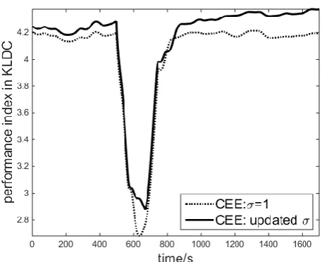
[image:19.595.175.407.338.521.2]20
Fig.7. Time profile of the performance index (9) used to update kernel size
4. Conclusions
In this paper, an adaptive NN-PID controller is proposed for the primary controller design in a cascade control system. To enhance the tracking performance for non-Gaussian and nonlinear stochastic systems, a new CEE performance index is proposed to train the NN-PID controller in the primary control loop, which combines the minimum entropy and the maximum cross correntropy of the tracking error. The kernel function for this entropy-based performance index is recursively updated by employing a receding horizon window technique. The training algorithm of the NN-PID controller is derived using the steepest descent approach, and its convergence conditions are investigated with the use of a linearisation technique.
This algorithm is applied to simulation study of superheated steam temperature control in an industrial-scale boiler system. The controller performances are investigated for several entropy-based metrics. Simulation results demonstrate with the proposed method, a balanced performance of reducing randomness and amplitude of tracking errors can be achieved conveniently.
[image:20.595.177.406.62.248.2]21
5. Acknowledgments
This work was supported by National Basic Research Program of China under Grant (973 Program, Grant No. 2011CB710706), the Natural Science Foundation of China (61503271, 61374052 and 61511130082) and Beijing (4142048). These are gratefully acknowledged.
6. References
[1] Liu, X.-J., Chan, C.: 'Neuro-fuzzy generalized predictive control of boiler steam temperature', IEEE Trans. Energy Convers., 2006, 21, (4), pp. 900-908
[2] Silva, R., Shirley, P., Lemos, J., Goncalves, A.: 'Adaptive regulation of super-heated steam temperature: a case study in an industrial boiler', Control Eng. Pract., 2000, 8, (12), pp. 1405-1415
[3] Zhang, J., Zhang, F., Ren, M., Hou, G., Fang, F.: 'Cascade control of superheated steam temperature with neuro-PID controller', ISA Trans., 2012, 51, (6), pp. 778-785
[4] Dash, P., Saikia, L. C., Sinha, N.: 'Automatic generation control of multi area thermal system using Bat algorithm optimized PD–PID cascade controller', Int. J. Elec. Power, 2015, 68, 364-372
[5] Son, Y. I., Kim, I. H., Choi, D. S., Shim, H.: 'Robust cascade control of electric motor drives using dual reduced-order PI observer', IEEE Trans. Ind. Electron., 2015, 62, (6), pp. 3672-3682
[6] Chai, S., Wang, L., Rogers, E.: 'A cascade MPC control structure for PMSM with speed ripple minimization',
IEEE Trans. Ind. Electron., 2013, 60, (8), pp. 2978-2987
[7] Errouissi, R., Ouhrouche, M., Chen, W.-H., Trzynadlowski, A. M.: 'Robust cascaded nonlinear predictive control of a permanent magnet synchronous motor with antiwindup compensator', IEEE Trans. Ind. Electron.,
2012, 59, (8), pp. 3078-3088
[8] Bocker, J., Freudenberg, B., The, A., Dieckerhoff, S.: 'Experimental comparison of model predictive control and cascaded control of the modular multilevel converter', IEEE Trans. Power Electron., 2015, 30, (1), pp. 422-430 [9] Chen, Z., Gao, W., Hu, J., Ye, X.: 'Closed-loop analysis and cascade control of a nonminimum phase boost
converter', IEEE Trans. Power Electron., 2011, 26, (4), pp. 1237-1252
[10] Abouloifa, A., Giri, F., Lachkar, I., et al.: 'Cascade nonlinear control of shunt active power filters with average performance analysis', Control Eng. Pract., 2014, 26, 211-221
[11] Huang, C., Bai, Y., Liu, X.: 'H-infinity state feedback control for a class of networked cascade control systems with uncertain delay', IEEE Trans. Ind. Informat., 2010, 6, (1), pp. 62-72
[12] Mathiyalagan, K., Park, J. H., Sakthivel, R.: 'New results on passivity-based H∞ control for networked cascade control systems with application to power plant boiler–turbine system', Nonlinear Anal-Hybri., 2015, 17, 56-69
[13] Du, Z., Yue, D., Hu, S.: 'H-infinity stabilization for singular networked cascade control systems with state delay and disturbance', IEEE Trans. Ind. Informat., 2014, 10, (2), pp. 882-894
[14] Li, C., Choudhury, M. S., Huang, B., Qian, F.: 'Frequency analysis and compensation of valve stiction in cascade control loops', J. Process Contr., 2014, 24, (11), pp. 1747-1760
[15] Todeschini, F., Corno, M., Panzani, G., Fiorenti, S., Savaresi, S. M.: 'Adaptive cascade control of a brake-by-wire actuator for sport motorcycles', IEEE/ASME Trans. Mechatronics, 2014, 20, (3), pp. 1310-1319
[16] Tschanz, F., Zentner, S., Onder, C. H., Guzzella, L.: 'Cascaded control of combustion and pollutant emissions in diesel engines', Control Eng. Pract., 2014, 29, 176-186
[17] Mehdi, N., Rehan, M., Malik, F. M., Bhatti, A. I., Tufail, M.: 'A novel anti-windup framework for cascade control systems: An application to underactuated mechanical systems', ISA Trans., 2014, 53, (3), pp. 802-815 [18] Guo, C., Song, Q., Cai, W.: 'A neural network assisted cascade control system for air handling unit', IEEE
Trans. Ind. Electron., 2007, 54, (1), pp. 620-628
[19] Dominici, M., Cortesão, R.: 'Cascade force control for autonomous beating heart motion compensation',
Control Eng. Pract., 2015, 37, 80-88
22
[21] Spall, J. C., Cristion, J. A.: 'Model-free control of nonlinear stochastic systems with discrete-time measurements', IEEE Trans. Autom. Control, 1998, 43, (9), pp. 1198-1210
[22] Xu, D., Jiang, B., Shi, P.: 'A novel model-free adaptive control design for multivariable industrial processes',
IEEE Trans. Autom. Control, 2014, 61, (11), pp. 6391-6398
[23] Wei, Q., Liu, D.: 'Data-driven neuro-optimal temperature control of water–gas shift reaction using stable iterative adaptive dynamic programming', IEEE Trans. Autom. Control, 2014, 61, (11), pp. 6399-6408
[24] Bu, X., Hou, Z., Yu, F., Wang, F.: 'Robust model free adaptive control with measurement disturbance', Control Theory Appl., 2012, 6, (9), pp. 1288-1296
[25] Tong, S.-C., Sui, S., Li, Y.-M.: 'Fuzzy adaptive output feedback control of MIMO nonlinear systems with partial tracking errors constrained', IEEE Trans. Fuzzy. Syst., 2015, 23, (4), pp. 729–742
[26] Liu, Y.-J., Tong, S.: 'Adaptive fuzzy identification and control for a class of nonlinear pure-feedback MIMO systems with unknown dead zones', IEEE Trans. Fuzzy. Syst., 2015, 23, (5), pp. 1387–1398
[27] Tong, S.-C., Zhang, L., Li, Y.-M.: 'Observed-based adaptive fuzzy decentralized tracking control for switched uncertain nonlinear large-scale systems with dead zones', IEEE Trans. Syst., Man, Cybern., Syst., 2016, 46, (1), pp. 37–47
[28] Tong, S.-C., Wang, T., Li, Y.-M., Zhang, H.-G.: 'Adaptive neural network output feedback control for stochastic nonlinear systems with unknown dead-zone and unmodeled dynamics', IEEE Trans. Cybern., 2014,
44, (6), pp. 910–921
[29] Liu, Y.-J., Tong, S.: 'Adaptive NN tracking control of uncertain nonlinear discrete-time systems with nonaffine dead-zone input', IEEE Trans. Cybern., 2015, 45, (3), pp. 497–505
[30] Liu, Y.-J., Tang, L., Tong, S., Chen, C. L. P.: 'Adaptive NN controller design for a class of nonlinear MIMO discrete-time systems', IEEE Trans. Neur. Net. Lear. Syst., 2015, 26, (5), pp. 1007–1018
[31] Chen, B., Zhu, Y., Hu, J.: 'Mean-square convergence analysis of ADALINE training with minimum error entropy criterion', IEEE Trans. Neural Netw., 2010, 21, (7), pp. 1168-1179
[32] Chen, B., Zhu, Y., Hu, J., Principe, J. C.: in 'System parameter identification: information criteria and algorithms' (Newnes, 2013, 1st edn).
[33] Erdogmus, D., Principe, J. C.: 'An error-entropy minimization algorithm for supervised training of nonlinear adaptive systems', IEEE Trans. Signal Process, 2002, 50, (7), pp. 1780-1786
[34] Principe, J. C.: in 'Information theoretic learning: Renyi's entropy and kernel perspectives' (Springer Science & Business Media, 2010, edn).
[35] Guo, L., Wang, H.: in 'Stochastic distribution control system design: a convex optimization approach' (Springer Science & Business Media, 2010, 1st edn).
[36] Yue, H., Wang, H.: 'Minimum entropy control of closed-loop tracking errors for dynamic stochastic systems',
IEEE Trans. Autom. Control, 2003, 48, (1), pp. 118-122
[37] Yue, H., Zhou, J., Wang, H.: 'Minimum entropy of B-spline PDF systems with mean constraint', Automatica,
2006, 42, (6), pp. 989-994
[38] Ren, M., Zhang, J., Wang, H.: 'Minimized tracking error randomness control for nonlinear multivariate and non-Gaussian systems using the generalized density evolution equation', IEEE Trans. Autom. Control, 2014, 59, (9), pp. 2486-2490
[39] Zhang, J., Ren, M., Wang, H.: 'Minimum entropy control for non-linear and non-Gaussian input and two-output dynamic stochastic systems', IET Control Theory Appl., 2012, 6, (15), pp. 2434-2441
[40] Ren, M., Zhang, J., Jiang, M., Yu, M., Xu, J.: 'Minimum entropy control for non-Gaussian stochastic
networked control systems and its application to a networked DC motor control system', IEEE Trans. Control Syst. Technol., 2015, 23, (1), pp. 406-411
[41] Zhang, X., Ren, X., Na, J., Zhang, B., Huang, H.: 'Adaptive nonlinear neuro-controller with an integrated evaluation algorithm for nonlinear active noise systems', J. Sound Vib., 2010, 329, (24), pp. 5005-5016 [42] Chen, H., Xing, G., Sun, H., Wang, H.: 'Brief paper-Indirect iterative learning control for robot manipulator
with non-Gaussian disturbances', IET Control Theory Appl., 2013, 7, (17), pp. 2090-2102
[43] Zhou, H., Bouyekhf, R., El Moudni, A.: 'Modeling and entropy based control of urban transportation network',
Control Eng. Pract., 2013, 21, (10), pp. 1369-1376
23