Identifying component modules

R I WHITFIELD, J S SMITH AND A H B DUFFY

University of Strathclyde, CAD Centre, DMEM, James Weir Building, 75 Montrose Street, Glasgow, UK, G1 1XJ

Abstract. A computer-based system for modelling component dependencies and identifying component modules is presented. A variation of the Dependency Structure Matrix (DSM) representation was used to model component dependencies. The system utilises a two-stage approach towards facilitating the identification of a hierarchical modular structure. The first stage calculates a value for a clustering criterion that may be used to group component dependencies together. A Genetic Algorithm is described to optimise the order of the components within the DSM with the focus of minimising the value of the clustering criterion to identify the most significant component groupings (modules) within the product structure. The second stage utilises a ‘Module Strength Indicator’ (MSI) function to determine a value representative of the degree of modularity of the component groupings. The application of this function to the DSM produces a ‘Module Structure Matrix’ (MSM) depicting the relative modularity of available component groupings within it. The approach enabled the identification of hierarchical modularity in the product structure without the requirement for any additional domain specific knowledge within the system. The system supports design by providing mechanisms to explicitly represent and utilise component and dependency knowledge to facilitate the non-trivial task of determining near-optimal component modules and representing product modularity.

1. Introduction

gained increasing prominence as a potential means to facilitate improved product architectures/platform design and re-use support (Smith et al. 2001a, Smith et al. 2001b).

Modular design involves the creation of product variants based on the configuration of a defined set of modules. Modules are commonly described as groups of ‘functionally’ or ‘structurally’ independent components (Sosale et al. 1997). The principal aim is to create variety, reduce complexity and maximise kinship in designs and across product families. The major benefits of a modular design include: efficient upgrades; reduced complexity; reduced costs; rapid product development, and, improved design knowledge structuring (Miller 1999, Muffato 1999, O’Grady et al. 1998). Despite the existing evidence regarding its benefits and the increased understanding of the capabilities of modularity as a design tool, ‘little work has been done on these research issues’ (O’Grady et al. 1998) and ‘modularity has been treated in the literature in an abstract form’ (Huang et al. 1998). That is, there is little aid in the form of tools, techniques and methodologies for practicing designers, and consequently, a need exists for approaches ‘to determine modules, represent modularity, and optimise modular design’ (Huang et al. 1998).

A number of algorithms exist that may be applied to the optimisation of modular design problems including simulated annealing (Kirkpatrick et al. 1983), Genetic Algorithms (GA) (Holland 1962) and Tabu search (Glover 1993). The optimisation algorithms tend to have a number of parameters that affect their performance and are intrinsically linked to the problem domain, for example, the annealing schedule for simulated annealing.

This paper demonstrates the application of a GA to component structure optimisation where the objective was to determine the optimum modular configuration for the design artefact. Modularisation research is discussed within Section 2 in order to identify the requirements for a modular identification system. The Dependency Structure Matrix (DSM) – Steward (1981) was used as the dependency modelling technique due to its generic applicability, ease of representation within a computer-based system, and, its quantifiable nature. The DSM modelling technique and system are described within Section 3. A multi-criteria GA was developed and adapted for application to this particular type of problem and is described within

Section 4. Section 5 defines the‘Module Strength Indicator’ (MSI)function

that is used to facilitate module identification and production of a ‘Module

2. Modularisation Research

The main characteristics that determine modularity have been defined as the degree of interaction/dependency between components both: within a module, and, of different modules (Ulrich et al. 1991, Kusiak et al. 1996).

The criteria for the optimal modular product structure can thus, be defined as the clustering of components such that the degree of interaction/dependency is:

• Maximised internally within groups (modules).

• Minimised externally between groups (modules).

The challenge for modular design research is to identify this optimal modular structure. Firstly, there is the requirement for the adequate modelling of component and interaction knowledge to support its analysis. Secondly, the resulting model must be optimised with respect to the above criteria. Finally, modules must be identified based on the results of the optimisation process.

A number of researchers have addressed the problem of modularising product designs. The modelling requirements are generally fulfilled using either interaction graphs (Kusiak et al. 1996) or matrix techniques (Blackenfelt 2001, Jarventausta et al. 2001, Salhieh et al. 1999, Sosale et al. 1997). Optimisation criteria and techniques vary between applications. For example, Salhieh and Kamrani (1999) utilised a P-median model to optimise the sum of component similarities, Jarventausta and Pulkkinen (2001) the Cluthill-McGee algorithm and Sosale et al. (1997) used a simulated annealing algorithm. Alternatively Blackenfelt (2001) based component groupings on their ability to fulfil the criteria of a series of strategic module drivers such as ‘styling’ or ‘the make or buy decision’. Despite the availability of varying methods to both model and optimise component and interaction knowledge, there are disparities with respect to the methods for the identification of modules within these optimised models. For example, in Jarventausta and Pulkkinen (2001), and Salhieh and Kamrani (1999) modules are identified manually by perusing an optimised matrix. In Sosale et al. (1997) the results of the optimisation are presented in a list of components each with a value indicating the module number to which the component is assigned. However, it is not clear from their published works (Sosale et al. 1997, Gu et al. 1997) how these modules are extracted from the optimised matrix. The rationale given for their module groupings would suggest that it is subject to manual interpretation of the matrix.

inter-dependencies between components. In such cases, the clustered matrix/graph may be densely populated and on first perusal yield no significant modules. Therefore, an alternative analysis of the optimised model would be required to facilitate module identification. Such analysis would conceivably require the utilisation of further resources such as domain specific knowledge. This would result in additional time and effort on the part of the human designer and/or the development of computational support systems. Further, when modules are readily identifiable, whether manually or automatically, it may not always be appropriate to return a list of definitive modules as suggested by Sosale et al. (1997). For example, what is modular from one perspective (e.g. assembly) may not be modular from another (e.g. maintenance) (Miller 1998). Thus, we see that the modular design problem is further complicated by the fact that differing modular configurations support different perspectives of the problem. In addition, the modular design may also exist over different hierarchical levels of the product structure. Thus, the inherent hierarchical modularity is not exposed when the outcome of the identification phase is presented as a list (Sosale et al. 1997) or as definitive module boundaries (Salhieh et al. 1999).

Given the above, the following must be determined in order to develop a means to facilitate improved module identification:

• Inherent modularity.

• Potentially differing modular configurations.

• Differing hierarchical levels of modularity in the product structure.

Our aim is to facilitate module identification with respect to the above modular requirements. The means of doing so is to combine the strengths of both the designer, in terms of their domain and problem specific knowledge, and of computer support, in terms of its advanced capabilities for rapid and precise analysis and calculation.

3. Dependency Structure Matrix

The Dependency Structure Matrix (DSM), also known as the Design Structure Matrix, has been extensively used to represent concepts such as: tasks, resources and parameters, as well as the inter-concept dependencies. The DSM is generic in nature, but due to its compactness, easily

quantifiable nature, and ability to represent most design activity

The DSM consists of a list of concepts (activities, functions, parts) that are represented in the same order in both the row and column of the matrix. The matrix part represents the dependencies between the concepts. Steward (1981) originally represented the dependencies in a binary form: 0 to indicate no dependency, and, 1 to indicate a dependency, however, the modelling technique has evolved to reflect a measure of the degree of dependency, termed its weight.

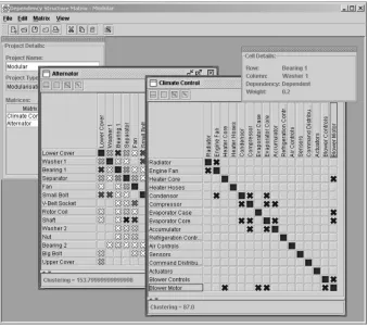
A DSM modelling and analysis system was constructed with the focus of providing mechanisms to enable the optimisation of the order of components with respect to a pre-determined clustering criterion – Figure 1.

The system allows the creation of a matrix containing any number of components with the matrix changing size automatically as components are added or removed. The dependencies between components are currently limited to representing a single type, e.g. a geometrical perspective, however, work is underway to enable the representation of multi-dimensional dependencies. Selecting a cell within the matrix will change the state of the dependency from either independent or dependent. The user may also change the weight of the dependency, which is reflected by its colour.

The order of the components within the matrix may be managed manually by dragging either of the rows or columns into a new position. The value for the clustering criterion is simultaneously re-calculated, assisting the user in the determination of an improved modular structure. Alternatively, the product structure may be optimised using one of the optimisation algorithms available within the optimisation module. The system can simultaneously manage the optimisation of multiple design artefacts although this will obviously take longer on a computer with a single processor.

4. Modular Structure Optimisation

A number of optimisation algorithms such as hill-climbing and simulated annealing were developed and tested within the optimisation of the order of components within the DSM (Whitfield 2001b). The difficulty in optimising the DSM lies in the number of combinations of possible component orders.

For example, a matrix containing 30 components has 6.652*1032 possible

combinations. An exhaustive search for this type of problem is clearly inappropriate. There is also a requirement for the optimisation technique to be able to deal with discrete, multi-modal, noisy and multi-criteria solution spaces that are common within the DSM (Todd 1997).

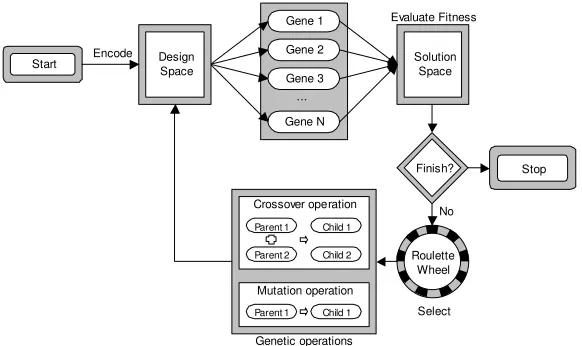
The general procedure for Genetic Algorithms developed by Goldberg (1989a), has been used to enable the evolution of optimal modular

structures. The objective of the GA in this particular application is to

minimise the value for the clustering criterion – Equation 1. Additional clustering criteria will be included to investigate other modular performance characteristics. The algorithm is illustrated within Figure 2.

Gene 1

Gene 3 Gene 2

Gene N

Mutation operation

Parent 1 Child 1 Parent 1

Parent 2 Child 1

Child 2

Crossover operation

Roulette Wheel

No ...

Evaluate Fitness

Select Finish?

Genetic operations

Encode _Solution

Space Design

Space Start

Stop

The system’s GA is generic in nature using object-oriented techniques and allows the encoding of a sequence of any type of concept. Within this application, the chromosome is initially encoded as a random order of components. This randomisation attempts to ensure that the chromosome represents a unique point in the solution space, such that the group of chromosomes are randomly distributed throughout – Figure 3. In the case of the DSM problem, the group of chromosomes, or population, represent orders of components that generally have a poor initial clustering criterion. The chromosomes are then evaluated within the DSM with respect to the criteria. Gene 1 Gene 2 Gene 3 Gene 4 Gene 5 Gene 6 Gene N … C om po nent 1 . C om po nent 5 . C om po nent 8 . C om po nent 4 . C om po nent 6 . C om po nent 3 . C om po nent 9 . C om po nent 2 . C om po nent 7 . C om pon e n t10 C om pon e n t7 . C om pon e n t2 . C om pon e n t4 . C om pon e n t1 . C om pon e n t8 . C om pon e n t5 . C om pon e n t6 . C o m pon e nt 10 . C om pon e n t3 . C om pon e n t9 C om ponent 9 . C om p onent 1 0 . C om ponent 5 . C om ponent 7 . C om ponent 6 . C om ponent 2 . C om ponent 1 . C om ponent 3 . C om ponent 8 . C om ponent 4 …

Figure 3. Genetic representation of component order.

A Roulette-wheel type selection procedure is used where each chromosome is given a portion of the wheel that is proportional to its performance (Goldberg 1989a). Chromosomes with higher performance characteristics therefore have a greater chance of surviving, although it is possible for lower performance chromosomes to be passed through to the next generation.

Table 1. Crossover operators encoded within GA.

Initial Description Reference

1PX One Point Crossover Murata & Ishibuchi (1994) 2PEX Two Point End Crossover Murata & Ishibuchi (1994) 2PCX Two Point Centre Crossover Murata & Ishibuchi (1994) 2PECX Two Point End/Centre Crossover Murata & Ishibuchi (1994)

PBX Position Based Crossover Syswerda (1991)

IPX Independent Position Crossover Murata & Ishibuchi (1994) PMX Partially Mapped Crossover Goldberg & Lingle (1985)

OX Ordered Crossover Davis (1985)

CX Cycle Crossover Oliver et al. (1987)

ERX Edge Recombination Crossover Whitley et al. (1989) EERX Enhanced Edge Recombination

Crossover

Starkweather et al. (1991)

SCX Subtour Chunks Crossover Greffenstette et al. (1985) AEX Alternating Edges Crossover Greffenstette et al. (1985)

IX Inversion Crossover Goldberg (1989b)

The new population is then re-evaluated with respect to the performance criteria. A check is made to determine whether the GA has completed a pre-determined number of generations, finishing if it has, otherwise repeating this evaluation, selection, crossover and mutation processes.

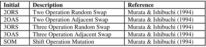
Table 2. Mutation operators encoded within GA.

Initial Description Reference

2ORS Two Operation Random Swap Murata & Ishibuchi (1994) 2OAS Two Operation Adjacent Swap Murata & Ishibuchi (1994) 3ORS Three Operation Random Swap Murata & Ishibuchi (1994) 3OAS Three Operation Adjacent Swap Murata & Ishibuchi (1994) SOM Shift Operation Mutation Murata & Ishibuchi (1994)

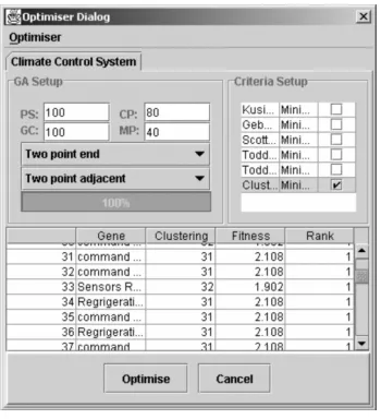
The parameters for the genetic algorithm and the optimisation criteria may be selected using the optimiser dialog shown within Figure 4. The population size, number of generations, crossover probability and mutation probability may be entered within the text fields. An indicator displays the genetic algorithm’s progress through the evaluation of the populations.

A previous investigation attempted to determine the parameters for generic combinatorial optimisation using GAs (Todd 1997), however research has demonstrated that the parameters for the GA are intrinsically tied to the domain (Whitfield et al. 2001a).

respectively was the most successful set-up for the GA. The population size and generation count were both set at 100.

Figure 4. Optimiser dialog.

Criteria may be selected for the basis of optimisation using the Criteria Set-up area of the optimisation dialog. The optimisation may be either single criterion or multi-criteria where the individual objectives are minimisation, maximisation, target value, or any combination.

After completion of the optimisation, a list of optimal component orders is displayed within the solution table. The list displays the component order, the values for the criteria selected, the fitness and the rank for each of the solutions. For multi-criteria problems, the genetic algorithm will produce a number of solutions that represent the trade-off between the criteria. Selecting one of the optimum solutions within the solution table will display the component ordering within the DSM.

The clustering criterion is represented within Equation 1. The DSM model may however have any number of criteria included to increase the diversity of the optimisation. Equation 1 represents the summation of the dependencies both above and below the leading-diagonal multiplied by their distance from the leading-diagonal on the basis of their weight. The focus of minimising the clustering criterion is therefore to get the dependencies as close to the leading diagonal as possible grouping component dependencies

together. Priority is automatically given towards higher weighted

dependencies.

(

)

(

)

! !

= N

i N

j j i wi j

Criterion lustering

1 1 ,

Where: Nis the number of components in the DSM,

iandjare the row and column indices, and

wi,jare the dependency weights.

The criteria values are automatically re-calculated and updated when new components are added to the matrix, or when component dependencies are changed, and are displayed within the criteria area.

5 Module Identification

A function was derived to assign a‘Module Strength Indicator’ (MSI)to all

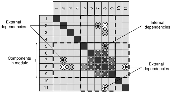
potential modules within the design artefact. The MSI function consists of two parts, Equations 2 and 3 below. Equation 2 provides the designer with the mean value of the internal dependencies within the module determined by the indices and represents the strength of the internal dependencies of a component grouping. Equation 3 determines a mean value for the external dependencies within the module and represents the strength of the external dependencies of the component grouping. The focus of the MSI function is towards identifying modules that have a maximum number of internal dependencies and a minimum number of external dependencies – Figure 5.

1

1

2

3

4

5

6

7

8

9

10

11

2 3 4 5 6 7 8 9 _{10 11}

External dependencies External

dependencies

Internal dependencies

Components in module

Figure 5. Internal and external dependencies of module.

(

)

(

)

! !

(

)

(

)

(

(

) (

)

)

, , 1 2 1 0 , , 2 2 2 2 1 1 2 1 n n n N w w n n n w w MSI N n i n n j i j j i n i n n j i j j i e − × − × + + − × × + =

! !

! !

MSI = − 4

Where; n1= index of first component in module, and

n2= index of last component in module.

Given a maximum dependency weight within the DSM of 1.0, the maximum MSI value that can be returned from Equation 4 is 1.0. This represents the strongest possible module solution, i.e. a module consisting entirely of maximum weight internal dependencies (1.0 from Equation 2), with no related external dependencies (0.0 from Equation 3). The system provides the functionality to allow the designer to specify module identification criteria. The designer can choose to: exclude external dependencies (use only Equation 2); normalise the MSI results, and, assign colours to incremental value ranges of the MSI. The system then traverses through the DSM calculating an MSI value for all possible modules.

The MSI technique results in an alternative representation of the DSM.

The resulting ‘Module Structure Matrix’ (MSM) depicts, as different

coloured cells, the relative modularity of all available component modules within it. Thus, the MSM exposes the boundaries of any existing modular structure based on the given dependencies. The MSM identifies inherent hierarchical modularity within highly constrained problems with densely populated dependency matrices that otherwise may not have been readily apparent. Further, as the coloured groupings represent different strengths of modularity the MSM reveals the inherent hierarchical modularity within the structure.

6 Case Studies

The module identification approach is demonstrated within two case studies. The studies, taken from published literature represent: a climate control system (Pimmler et al. 1994), and, an alternator (Sosale et al. 1997). The climate control example depicts the components and their dependencies from a material perspective. The alternator case depicts dependencies based on the re-use and recycling life-phase of the artefact’s components.

6.1 CLIMATE CONTROL SYSTEM

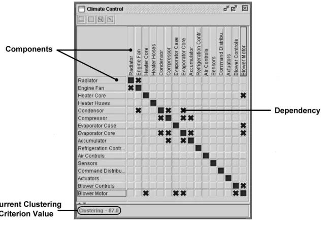
Figure 6 presents a DSM for a climate control system. The system’s components are represented by the same arbitrary structure in both the column and rows. The crosses in the central part of the matrix represent the dependencies between the components, which in this case, are all equally weighted. The current value for the clustering criterion is shown in the left-hand bottom corner of the box. The value for the clustering criterion for this structure is 87.0.

Figure 6. Climate control system DSM.

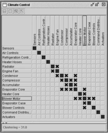
Figure 7. Optimised climate control system DSM.

However, the potential modular configurations and the applicable hierarchical modularity within the given solution are not apparent from the optimised DSM. The MSI function was applied to highlight modular configurations and hierarchical modularity. The resulting MSM is presented in Figure 8. This matrix was obtained through the application of Equation 4 to the DSM within Figure 7 with normalised results. The matrix provides a mechanism from which to identify potential modules of varying modular strength represented by differing colours. The results indicate that there are a number of modular configurations and that a hierarchical modularity exists within the structure.

Figure 8. Climate control system MSM.

Table 3a. Module Catalogue for Climate Control System.

Modular Strength Module Components

1.0 M1 Radiator, Engine Fan

M2 Condenser, Compressor

M3 Compressor, Accumulator, Evaporator Core

M4 Heater Core, Blower Motor

0.9

M5 Blower Motor, Evaporator Case

0.8 M6 Components within M2and M3

M7 Components within M4and M5

0.7

M8 Components within M5and Blower Controls

M9 Components within M8and Heater Core

M10 Components within M4and Evaporator Core

0.6

M11 Components within M6and Engine Fan

M12 Components within M11and Radiator

M13 Components within M6and M7

0.5

M14 Components within M7, Evaporator Core and

Blower Controls

M15 Components within M1, M6, Refrigeration

Controls and Heater Hoses

M16 Components within M1and M13and Blower

Controls 0.4

M17 Components within M13, Blower Controls and

Command Distributor

Table 3b Hierarchical Module Configuration Example

Configuration Module Components

M1 Engine Fan, Radiator

M6 Condenser, Compressor, Accumulator,

Evaporator Core. Level i

M7 Heater Core, Evaporator Case, Blower Motor

Level ii M13 M6and M7

Level iii M16 M1, M13and Blower Controls

Level iv M18 M16,Sensors, Air Controls, Refrigeration

Controls, Heater Hoses, Command Distributor and Actuators

6.2 ALTERNATOR

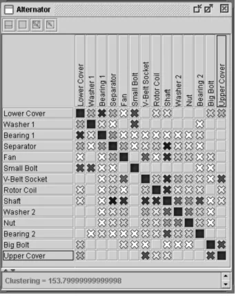
The DSM for an Alternator is presented in Figure 9. Again, the components are represented in an arbitrary structure and the crosses represent the dependencies between the components.

Figure 9. Alternator DSM.

The weightings were calculated as the sum of a number of different life-phase aspects such as: maintenance, upgrading, and reconfiguration. The alternator case therefore represents a more highly constrained problem than that of the climate control system, as indicated by the densely populated matrix. The value of the clustering criterion for this structure is 153.8.

approximately 23%. Without further analysis, it is difficult to clearly identify any significant component groupings within the optimised DSM. The MSI function is applied and the resulting MSM is shown in Figure 11.

Figure 10. Optimised alternator DSM.

Again the results are normalised and are based on the application of Equation 4. It is apparent from Figure 11 that there are a number of strong module groupings and hierarchical levels within the artefact.

Table 4a catalogues all available modules within the structure at the differing module strengths highlighted by the MSM. Such modularity is not immediately evident from the dependencies displayed within the optimised DSM - Figure 10.

Table 4. Module Catalogue for Alternator.

Modular Strength Module Components

1.0 M1 Lower Cover, Bearing 1

M2 Upper Cover, Big Bolt

M3 Small Bolt, Washer 1

0.9

M4 Small Bolt, Lower Cover

M5 Components within M3and M4

M6 Rotor Coil, Shaft

M7 Shaft, Fan

0.7

M8 V Belt Socket, Upper Cover

0.6 M9 Components within M1and M5

M10 Components within M1and Separator

M11 Components within M6, Separator and Bearing

2 0.5

M12 Components within M6, M7, Washer 2, Nut and

V Belt Socket

M13 Components within M2and M8

M14 Components within M9and Separator

M15 Components within M11, M12and Bearing 1

0.4

M16 Components within M11, M12and Upper Cover

0.3 M17 All

As with the Climate Control case the designer can utilise this module catalogue and the MSM to identify a number of differing modular configurations within the product structure.

developed to support new design. As such the system can be applied to design viewpoints other than structural, i.e. functional, and working principles (means). Further ‘between viewpoint’ mapping mechanisms are currently under investigation to allow the principles of modularity to be applied throughout the evolution of a new design.

Similarly, the system currently represents dependencies for a single ‘perspective’ of any viewpoint such as the physical relationships of components. Work is underway to extend the functionality to enable the representation of multiple perspectives within a single matrix, for example, the representation of dependencies from energy, material, and information perspectives. This functionality provides the means to simultaneously consider more than one perspective in the determination of inherent hierarchical modularity.

7 Conclusions

A generic system for representing the component structure and inter-component dependencies for design artefacts has been presented. The system evaluates a clustering criterion using the dependencies for any given structure of components. The system also incorporates a genetic algorithm to optimise the clustering objective through the re-ordering of the components.

A ‘Module Strength Indicator’ (MSI) was derived based on the criteria for an optimal modular structure, which is defined as the maximisation of internal dependencies and the minimisation of external dependencies. The

application of the MSI to the DSM resulted with a ‘Modular Structure

Matrix’ (MSM), which represents inherent hierarchical modularity within the product structure.

The system’s functionality was demonstrated through two case studies and illustrated the ability to facilitate the identification of near-optimal component modules without the need for any other domain or artefact specific knowledge. The results of both case studies identified similar module configurations as those defined in the original publications. Minor differences between modules identified were due to the application of domain specific knowledge by the authors of the original research. Inclusion of this knowledge within the original matrices would have influenced the results accordingly.

Acknowledgements

The authors gratefully acknowledge the support given by the Engineering

and Physical Science Research Council who provided the grant

RES/4741/0929 and postgraduate studentship no.98319349.

References

Andreasen, M.M., A. Duffy, and N.H. Mortensen. Relation Types in Machine Systems. in

WDK Workshop on Product Structuring. 1995. Delft University of Technology, Delft, The Netherlands.

Andreasen, M.M., C.T. Hansen, and N.H. Mortensen. The Structuring of Products and

Product Programmes. in 2nd WDK Workshop on Product Structuring. 1996. Delft

University of Technology, Delft, The Netherlands.

Blackenfelt, M.: 2001, Modularisation by relational matrices – a method for consideration of

strategic and functional aspects, inDesign for Configuration – a debate based on the 5th

WDK Workshop on Product Structuring,Riitahuhta, A. and Pulkkinen, A (eds), 134-152, Springer.

Coates, G., Duffy, A.H.B., Hills, W. and Whitfield, R.I.: 2000, A Generic Coordination

Approach Applied to a Manufacturing Environment, Journal of Materials Processing

Technology,107:404-411.

Davis, L.: 1985, Job Shop Scheduling and Genetic Algorithms, Proceedings of the First

International Conference on Genetic Algorithms and their Applications, Lawrence Erlbaum Associates, Hillsdale, NJ, USA, pp. 136-140.

Elgard P. and Miller, T. D.: 1998, Designing product families, Design for Integration in

Manufacturing in Proceedings of the13th IPS Research Seminar, Aalborg University, Fugsloe.

Eppinger, S.D., Whitney, D.E., Smith, R.P. and Gebala, D.A.: 1994, A model-based method

for organizing tasks in product development,Research in Engineering Design,6:1-13.

Erens, F. and Vershulst, K.: Managing System Design. in WDK Workshop on Product

Structuring. 1995. Delft University of Technology, Delft, The Netherlands.

Erens, F. and Vershulst, K.: 1996, Architectures for product families,in 2ndWDK Workshop

on Product Structuring,Delft University of Technology, Delft, The Netherlands.

Gershenson, J. K., Jagannath Prasad, G. and Allamneni, S.: 1999, Modular product design: a

life-cycle View,Journal of Integrated Design and Process Science,3(4).

Glover, F. and Laguna, M.: 1993, Tabu search, in Modern Heuristic Techniques for

Combinatorial Problems, Reeves CR ed. Blackwell Scientific Publications, Oxford, UK, pp. 70-150.

Goldberg, D.E. and Lingle, R.: 1985, Alleles, Loci and the Travelling Salesman Problem,

Proceedings of the First International Conference on Genetic Algorithms and Their Applications, Lawrence Erlbaum Associates, Hillsdale, NJ, USA, pp. 154-159.

Goldberg, D.E.: 1989a,Genetic Algorithms in Search, Optimisation and Machine Learning,

Addison-Wesley, Massachusetts, USA.

Goldberg, D.E.: 1989b, Sizing populations for serial and parallel Genetic Algorithms,

Proceedings of the Third International Conference on Genetic Algorithms, Morgan Kaufmann Publishers, CA, USA, pp. 70-79.

Gonzalz-Zugasti, J.P., and Otto, K.N.: 2000, Modular platform based product family design,

Greffenstette, J.J., Gopal, R., Rosmaita, B. and VanGucht, D.: 1985, Genetic Algorithms for

the Travelling Salesman Problem,Proceedings of the First International Conference on

Genetic Algorithms and Their Applications, Lawrence Erlbaum Associates, Hillsdale, NJ, USA, pp. 160-168.

Gu, P., Hashemian, M. and Sosale, S.: 1997, An integrated modular design methodology for

life-cycle engineering,Manufacturing Technology CIRP Annals,46(I), 71-74.

Holland, J.H.: 1962, Outline for a Logical Theory of Adaptive Systems,Joint Association of

Computing Machinery,9:297-314.

Huang, C. and Kusiak, A.: 1998, Modularity in design of products and systems, in

Transactions on Systems, Man and Cybernetics Part A – systems and humans, 28(1), IEEE.

Järventausta, S. and Pulkkinen, A.: 2001, Enhancing product modularisation with multiple

views of decomposition and clustering, inDesign for Configuration – a debate based on

the 5thWDK Workshop on Product Structuring,Riitahuhta, A. and Pulkkinen, A (eds), 153-168, Springer.

Jiao, J. and Tseng, M. M.: 1999, A methodology for developing product family architecture

for mass customisation,journal of intelligent manufacturing,12, 3-20, Kluwer Academic

Publishers.

Kirkpatrick, S., Gelatt, C.D. and Vecchi, M.P.: 1983, Optimisation by simulated annealing,

Science,220(4598):671-680.

Kusiak, A. and Park, K. 1990, Concurrent Engineering: Decomposition and Scheduling of

Design Activities,International Journal of Production Research,28(10):1883-1900.

Kusiak, A. and Huang, C.: 1996, Development of modular products,IEEE Transactions on

Components, Packaging and Manufacturing Technology, Part A, 19(4), December.

Minsk ML (1990) “ Process models for cultural integration”, Journal of Culture,

11(4):49–58.

Miller, T.D. and Elgard P.: 1998, Defining modules, modularity and modularisation,Design

for Integration in Manufacturing, Proceedings of the 13th IPS Research Seminar, Fugsloe, Aalborg University.

Miller, T.D.: 1999, Modular engineering of production plants,International Conference on

Engineering Design,Munich.

Muffato, M.: 1999, Introducing a platform strategy in product development,in International

Journal of Production Economics,60-61, 145-153, Elsevier Science.

Murata, T. and Ishibuchi, H.: 1994, Performance evaluation of Genetic Algorithms for flow

shop scheduling problems,Proceedings of the First IEEE Conference on Evolutionary

Computation,2:812-817.

O’Grady, P. and Liang, W.: 1998, An object oriented approach to design with modules,

Computer Integrated Manufacturing Systems,11(4), 267-283, Elsevier Science Ltd. Oliver I.M., Smith, C.J. and Holland J.R.C.: 1987, A study of permutation crossovers on the

Travelling Salesman Problem, Proceedings of the Second International Conference on

Genetic Algorithms and their Applications, pp. 225-230.

Otto, K.: 2001, A process for modularising product families, in Proceedings of the

International Conference on Engineering Design,August 21-23.

Pimmler, T.U. and Eppinger, S.D.: 1994, Integration analysis of product decompositions, Proceedings of the ASME Sixth International Conference on Design

Theory and Methodology, Minneapolis, MN, Sept., 1994. Also, M.I.T. Sloan School of Management, Cambridge, MA, Working Paper no. 3690-94-MS, May 1994.

Salheih, S. M. and Kamrani, A. K.: 1999, Macro level product development using design for

modularity, Robotics and Computer Integrated-Manufacturing, 15, 319-329, Elsevier

Smith, J.S. and Duffy A.H.B.: 2001a, Modularity in support of design for re-use, in the International Conference of Engineering Design, ICED, Glasgow, August 21-23.

Smith, J.S. and Duffy A.H.B.: 2001b, Product structuring for design re-use, in Design for

Configuration – a debate based on the 5th _{WDK Workshop on Product Structuring,}

Riitahuhta, A. and Pulkkinen, A (eds), 83-100, Springer.

Sosale, S., Hashemian, M. and Gu, P.: 1997, Product modularisation for re-use and recycling,

in Concurrent Product Design and Environmentally Conscious Manufacturing, DE 94,

ASME.

Starkweather, T., McDaniel, S., Mathias, K., Whitley, D. and Whitley, C.: 1991, A

comparison of genetic sequencing operators, Proceedings of the Fourth International

Conference on Genetic Algorithms, San Mateo, CA, USA, pp. 69-76.

Steward, D.V.: 1981, The design structure system: a method for managing the design of

complex systems,IEEE Trans. Engineering Management,28:71-74.

Suh, N.P.: 1990, The principles of design, Oxford U.K., Oxford University Press.

Ulrich, K. and Tung, K.: 1991, Fundamentals of product modularity, in Issues in

Design/Manufacture Integration,Sharon, A. (ed), DE39, 73-79, ASME.

Syswerda, G.: 1991, Scheduling optimisation using Genetic Algorithms, in Handbook of

Genetic Algorithms, L. Davis ed. Van Nostrand Reinhold, pp. 332-349.

Todd, D.: 1997, Multiple Criteria Genetic Algorithms in Engineering Design and Operation, Ph.D. Thesis, Engineering Design Centre, University of Newcastle upon Tyne, UK. Whitfield, R.I., Duffy, A.H.B., Coates, G. and Hills W.: 2001a, Efficient process

optimisation, submitted to Journal of Concurrent Engineering Research and

Applications.

Whitfield, R.I., 2001b, “Effective Combinatorial Optimisation”, CAD Centre internal report, CADC/01-06/R/03, DMEM, University of Strathclyde.

Whitley, D., Starkweather, T. and Fuquay, D.: 1989, Scheduling problems and the Travelling

Salesman: The Genetic Edge Recombination Operator, Proceedings of the Third

International Conference on Genetic Algorithms, Morgan Kaufmann, pp.133-140. Zamirowski, E.J. and Otto, K.N.: 1999, Identifying product portfolio architecture modularity

using function and variety heuristics,in Proceedings of the 11thInternational Conference

on Design Theory and Methodology,Design Engineering Technical Conference, ASME. Zhang, Y.: Computer-based modelling and management for current working knowledge