Spatial Deep Networks for Outdoor Scene Classification

Scene Classification

Cong Dong

B. Eng. (Honours)

Australian National University

July 2015

A thesis submitted for the degree of Master of Philosophy at The Australian National University

Conclusion

While far from perfect, the Convention

codifies fundamental principles and

establishes mechanisms needed to

adapt management of international

rivers to climate change

.

Governing international watercourses

in an era of climate change:

Dr Jamie Pittock

Crawford School of Economics & Government The Australian National University Canberra, ACT 0200, Australia

[email protected]

Ms Flavia Loures

World Wildlife Fund Washington, DC United States of America

[email protected]

References:

Loures, F., Rieu-Clarke, A., & Vercambre, M. (2008). Everything you need to know about the UN Watercourses Convention. Gland, Switzerland: WWF International.

Pittock, J., Loures, F., & Patterson, M. (submitted). Governing transboundary rivers in an era of climate change. In: The UN Watercourses Convention in force: Strengthening international law for transboundary water management.

Dam on the Mekong River in China © U. Collier. Dam developments would be governed by the Convention

Assessment of the extent to which the Convention’s provisions may facilitate

adaptive management of international watercourses with climate change.

Assessing the UN Watercourses Convention

Climate change will alter the stationary hydrology

that underpins the many existing international

river agreements.

In our research, ten principles are identified for

adaptive management of shared rivers.

Assessing the Convention, it has effective

provisions for subsidiarity, equitable use, no

harm, dispute settlement, information and

communication.

The Convention is silent on funding, conjunctive

management with groundwater and revision of

its provisions.

Further institutional reforms are needed to

enhance the Convention’s governance.

Waters shared between nations

There are 276 rivers are shared between two or more countries. Shared river basins contain 60% of surface water flow, 50% of

the land surface and 40% of the world’s population.

These shared waters generate critical ecosystem services for humanity but are degrading.

Climate change will greatly exacerbate existing risks to water security.

Many institutions exist for the management of transboundary waters at different scales.

However, only 40% of shared rivers are managed under treaties and 80% of agreements involve only two nations rather than all basin states.

Importantly, most treaties lack vital mechanisms required for effective adaptive management.

UN Watercourses Convention

The Convention on the Law of the Non-Navigational Uses of International Watercourses (New York, 1997) –“the

Convention” - codifies common measures for cooperative management of shared waters.

Primarily the Convention provides for equitable use balanced by an obligation for states to do no significant harm.

After 37 years of negotiations the Convention was adopted in a UN General Assembly vote: 106 in favour, 57 absent or

abstained, 3 against.

As at March 2012 there are ratifications from 24 nations plus pledges from Denmark and Luxembourg.

Only 9 more ratifications are required for the Convention’s entry

into force.

Cooperative management of shared waters

Can the Convention aid climate change adaptation?

Computer Vision Group

Research School of Engineering

Declaration

The contents of this thesis are the results of original research and have not been submitted for a higher degree to any other university or institution.

The research work presented in this dissertation is my own and it is supervised by Dr. Jose M. Alvarez.

Cong Dong

College of Engineering and Computer Science, The Australian National University,

Canberra, ACT 2601, Australia.

I would like to express the deepest gratitude to my supervisor Dr. Jose M. Al-varez for his continuous support, understanding and encouragement throughout my MPhil study and related research. His guidance helped me in all the time of research and writing of this thesis. Without his patience and opportune counsel, the work presented in this thesis would have been a frustrating pursuit.

My sincere thanks also go to Prof. Andrew Y. Ng for his free online resources regarding Unsupervised Feature Learning and Deep Learning tutorials and Ma-chine Learning courses which provide me significant opportunities to learn essential knowledge about various deep learning techniques. Without the precious support from these resources, it would not be possible to conduct this research.

I would also like to thank the Computer Vision Discussion Group in ANU which gives me opportunities to discuss with other computer vision researchers and students. Their insightful ideas were valued greatly.

Last but not the least, I would like to thank my parents and girl friend for their unconditional love, spiritual support and continuous encouragement throughout my study and my life in general.

Abstract

Scene classification has become an increasingly popular topic in computer vision. The techniques for scene classification can be widely used in many other aspects, such as detection, action recognition, and content-based image retrieval. Recently, the stationary property of images has been leveraged in conjunction with convo-lutional networks to perform classification tasks. In the existing approach, one random patch is extracted from each training image to learn filters for convolu-tional processes. However, feature learning only from one random patch per image is not robust because patches selected from di↵erent areas of an image may con-tain distinct scene objects which make the features of these patches have di↵erent descriptive power. In this dissertation, focusing on deep learning techniques, we propose a multi-scale network that utilizes multiple random patches and di↵erent patch dimensions to learn feature representations for images in order to improve the existing approach.

Despite the much better performance the multi-scale network can achieve than the existing approach, lacking of local features and the spatial layout is one of the core limitations of both methods. Therefore, we propose a novel Spatial Deep Network (SDN) to further enhance the existing approach by exploiting the spatial layout of the image and constraining the random patch extraction to be performed in di↵erent areas of the image so as to e↵ectively restrict the patches to hold the necessary characteristics of di↵erent image areas. In this way, SDN yields compact but discriminative features that incorporate both global descriptors and the local spatial information for images. Experiment results show that SDN considerably exceeds the existing approach and multi-scale networks and achieves competitive performance with some widely used classification techniques on the OT dataset (developed by Oliva and Torralba). In order to evaluate the robustness of the proposed SDN, we also apply it to the content-based image retrieval on the Holidays dataset, where our features attain much better retrieval performance but have much lower feature dimensions compared to other state-of-the-art feature descriptors.

AE Auto-Encoders AI Artificial Intelligence

BFGS Broyden-Fletcher-Goldfarb-Shanno BoF Bag-of-Features

BP Back-propagation

CNN Convolutional Neural Networks DBN Deep Belief Networks

FK Fisher Kernel FV Fisher Vector

KNN K-Nearest Neighbors L-BFGS Limited-memory BFGS NN Neural Networks

PCA Principal Component Analysis RBM Restricted Boltzmann Machines ReLU Rectified Linear Units

SAE Stacked Auto-Encoder SGD Stochastic Gradient Descent SH Spectral Hashing

SIFT Scale-Invariant Feature Transform SP Spatial Pyramid

SVM Support Vector Machines

VLAD Vector of Locally Aggregated Descriptors

Notations and Symbols

weight decay term

✓ parameter set

W weight matrix

b bias term

Ln n-th layer

J overall cost error term

⇤ 2D convolution operation ⌃ covariance matrix

U eigenvector matrix

I identity matrix (_·) activation function

d(_·) absolute distance 1_{·} indicator function

Declaration i

Acknowledgements ii

Abstract iii

List of Acronyms iv

Notations and Symbols v

1 Introduction 1

1.1 Scene Classification . . . 3

1.2 Deep Learning . . . 6

1.3 Motivation . . . 7

1.4 Main Contributions . . . 9

1.5 Outline . . . 10

2 Background for Feature Learning and Scene Classification 11 2.1 Auto-Encoders . . . 11

2.1.1 Framework of Auto-Encoders . . . 12

2.1.2 Feedforward Pass . . . 13

2.1.3 Back-propagation . . . 14

2.1.4 Optimization Algorithms . . . 17

2.2 Classifiers . . . 18

2.2.1 Softmax . . . 18

2.2.2 K-Nearest Neighbors . . . 20

2.2.3 Support Vector Machines . . . 22

2.3 Stacked Auto-Encoders and Greedy Layer-wise Training . . . 26

2.4 Convolutional Neural Networks . . . 28

2.4.1 Feedforward Pass . . . 29

2.4.2 Back-propagation . . . 32

Contents vii

2.5 Other Related Techniques . . . 34

2.5.1 Principal Component Analysis . . . 34

2.5.2 Whitening . . . 35

3 Multi-scale Networks for Scene Classification 37 3.1 Applied Techniques . . . 37

3.2 Datasets . . . 40

3.3 Experiment Settings . . . 42

3.4 Experiments and Results Analysis . . . 44

3.4.1 Experiments with Auto-Encoders . . . 44

3.4.2 Experiments with Stacked Auto-Encoders . . . 49

3.4.3 Experiments with Convolutional Neural Networks . . . 49

3.4.4 Experiments with Baseline Approach . . . 50

3.4.5 Comparison among Feature Learning Techniques . . . 50

3.4.6 Experiments with Proposed Multi-scale Networks . . . 51

3.5 Conclusions . . . 55

4 Spatial Deep Networks for Feature Learning 56 4.1 Spatial Deep Networks . . . 57

4.2 Experiment settings . . . 60

4.3 Experiments for Classification . . . 60

4.3.1 One/two-level SDN with One Convolutional Layer . . . 60

4.3.2 One/two-level SDN with Three Convolutional Layers . . . . 62

4.3.3 Comparison between Feature Combination Strategies . . . . 63

4.3.4 Comparison with Other Methods . . . 64

4.4 Experiments for Image Retrieval . . . 65

4.5 Conclusions . . . 66

5 Conclusions and Future Work 68 5.1 Conclusions . . . 68

5.2 Future Work . . . 69

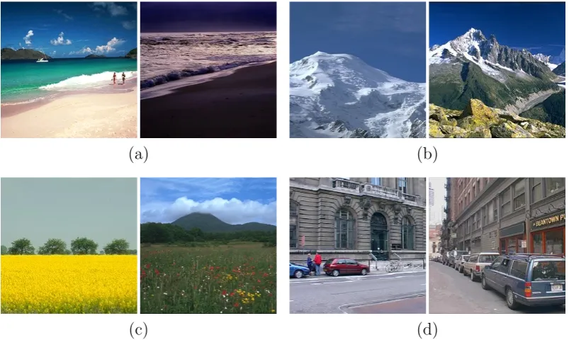
1.1 Challenges of scene recognition are: (a) illumination changes, (b) scale variations, (c) intra-class variability, and (d) inter-class simi-larities (in (d), the class of left image is ‘insidecity’, class of the right image is ‘street’). . . 2 1.2 Three-level Spatial Pyramid toy example: There are three feature

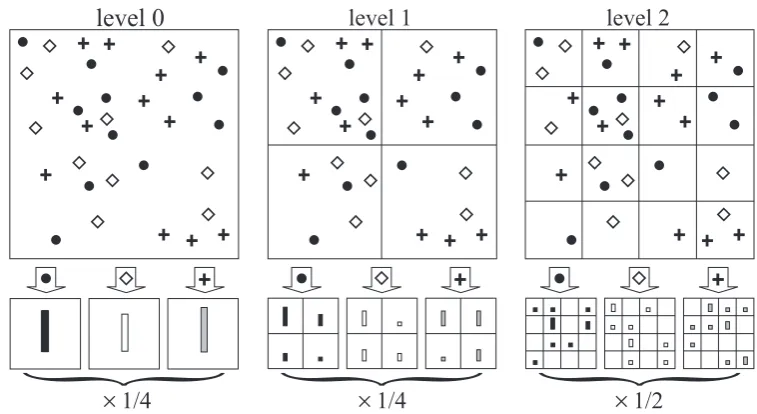
types: circles, diamonds, and crosses. Initially, partition image into three di↵erent level of resolution. Then, count the features found at each level of resolution. Finally, compute the final spatial histogram. 4 1.3 Convolutional Neural Network (CNN) structure of LeNet-5 used for

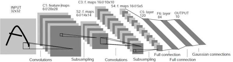
digits recognition. Each plane in the structure is a feature map whose weights are constrained to be identical. . . 8

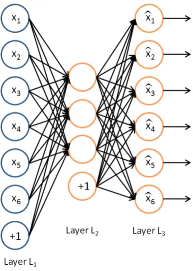
2.1 An example of 1-hidden-layer Auto-Encoder network. . . 12 2.2 Plots of sigmoid function and tanh function. . . 14 2.3 Sample plot of K-Nearest Neighbors criteria where k = 4 and the

training examples have two di↵erent labels, ‘Class A’ and ‘Class B’. 21 2.4 An example of linear separating hyperplane for the separable case in

2-dimensional space. The maximum margin distance is shown. The support vectors are those dots and circles, which define the margin of maximum separation between two classes. . . 24 2.5 Kernel machines used to compute a non-linearly separable function

into a higher dimension linearly separable function. . . 26 2.6 An example of convolutional layer. . . 30

3.1 Structure and feature learning procedures of proposed multi-scale networks. . . 39 3.2 Sample images from the OT dataset. . . 41 3.3 Sample images from the Holidays dataset. . . 42 3.4 An example of original image and its Gaussian Blurred image. . . . 46 3.5 PCA plots for 50D and 200D features: Variance VS. Components. . 48

List of Figures ix

3.6 Overall cost VS. Optimization iterations. . . 49

3.1 Accuracy of di↵erent scale reduction methods and image sizes. . . . 45

3.2 Accuracy of di↵erent distance metrics and AE structures. . . 47

3.3 Accuracy of di↵erent voting criteria and AE structures. . . 47

3.4 Comparison among AE, SAE, CNN, and baseline approach. . . 51

3.5 Results of di↵erent classification methods. . . 52

3.6 Results of di↵erent structures of SAE for dimension reduction. . . . 52

3.7 Results of di↵erent number of patches per training image. . . 53

3.8 Accuracy of di↵erent image sizes and patch sizes. . . 53

3.9 Results of less number of kernels and combined features. . . 54

3.10 Comparison between other techniques and proposed methods. . . . 55

4.1 Results of SDN with one convolutional layer. . . 62

4.2 Results of SDN with three convolutional layers. . . 63

4.3 Comparison of feature combination strategies. . . 64

4.4 Comparison with state-of-the-art techniques. . . 64

4.5 Comparison of features with the same dimension. . . 65

4.6 Comparison with state-of-the-art techniques. . . 66

Chapter 1

Introduction

Scene classification has become an increasingly popular topic in computer vision, which aims to categorize each test image and assign them to one of several scene types (mountain, forest, coast, city, etc.). E↵ective solutions to scene classification can be widely used in many other aspects, such as detection, action recognition, and content-based image retrieval. According to [1], scene classification is one of the most appealing yet challenging topics due to the high ambiguity and variability shown in the content of scene images, especially when images are in highly diverse. The challenges behind can be summarized as illumination changes and scale vari-ations, and also intra-class variabilities and inter-class similarities [2]. Figure 1.1 shows image examples of these challenges from the OT dataset (a scene dataset developed by Oliva and Torralba [3]). Therefore, learning good feature representa-tions for scene images is crucial for scene classification tasks.

In the past decades, machine learning has experienced an extraordinary ex-pansion and obtained an unprecedented popularity in many areas, including scene classification [4]. It is to build computer programs that are able to generate new knowledge or to improve knowledge already processed by using input informa-tion. However, the choice of data representation employed has significant influ-ences on the performance of many machine learning methods. For this reason, the intelligence behind the machine learning algorithms has shifted to designing ef-fective preprocessing pipelines and human-engineered feature extraction strategies to support certain machine learning tasks. Although such feature engineering is important, it can be challenging since it is labour-intensive and highly application-dependent [5, 6].

In order to expand the scope and ease of applicability of machine learning, it is highly desirable to make learning algorithms less dependent on the feature engi-neering [5]. Deep learning, a subfield of machine learning, was kick-started in the

(a) (b)

(c) (d)

Figure 1.1: Challenges of scene recognition are: (a) illumination changes, (b) scale variations, (c) intra-class variability, and (d) inter-class similarities (in (d), the class of left image is ‘insidecity’, class of the right image is ‘street’).

year of 2006 by a few research groups, especially Geo↵Hinton’s group who initially introduced Deep Belief Networks (DBNs) [7]. DBNs are a kind of deep networks that focus on stacking unsupervised feature learning algorithms to generate deeper representations for input data. Deep learning was proposed in order to move ma-chine learning systems towards automatically discovering multiple-level informa-tion representainforma-tions which contain higher-level features to represent more abstract concepts of information [5]. Since 2006, deep learning has seen rapid growth and has been applied with significant success in many traditional Artificial Intelligence (AI) applications, such as classification tasks [8,9], regression tasks [10], dimension reduction [11], object segmentation [12], information retrieval [13], robotics [14], natural language processing [15, 16], etc.

1.1 Scene Classification 3

1.1

Scene Classification

Despite the challenges behind scene classification, it is claimed that the human observer can deal with a number of visual tasks, like scene classification, with only around 100ms. This performance is attributed to the ability of a human to fast extraction the ‘gist’ of scenes without needing to perceive the object appeared in the scene [17]. Additionally, according to [18], a good feature representation for recognition tasks, such as scene classification, should have three properties:

• The capacity to achieve good performance for recognition tasks.

• Computational efficiency during generating the representations.

• Low demand on memory usage of representations.

To learn good feature representations and achieve scene classification with human-level performance, researchers have been making great e↵orts over the years. Some methods for scene classification follow the paradigm of describing images with a set of low-level attributes, such as color, texture, shape, and layout [19]. In spite of good performance these approaches can achieve, they lack intermediate image representations (such as the presence of sky, road, building, or other semantic con-cepts), which can be significantly valuable when doing scene classification.

In order to take advantage of intermediate representations, Bag-of-Features (BoF) proposed in [20] is one of the most popular and e↵ective approaches to model scenes, which is to quantize invariant local features into a set of visual words. The process can be summarized as follows:

- Local Features: To represent the image, descriptors are extracted based on

the interest-point detector technique [21]. Among di↵erent kinds of descrip-tors, SIFT (Scale-Invariant Feature Transform) proposed by [22] is one of the most commonly applied methods, which has the property to be invariant to rotations, scales, translations and small distortions of the original image.

- Codebook Representation: The other essential aspect of BoF is the codebook

get the following definition of a

pyramid match kernel

:

L

₍

_{X, Y}

₎

₌

I

+

L

_X

=0

1

2

I

I

+1

₍₂₎

=

1

2

I

0

₊

L

X

=1

1

2

I

.

(3)

Both the histogram intersection and the pyramid match

ker-nel are Mercer kerker-nels [7].

3.2. Spatial Matching Scheme

As introduced in [7], a pyramid match kernel works

with an orderless image representation. It allows for

pre-cise matching of two collections of features in a

high-dimensional appearance space, but discards all spatial

in-formation. This paper advocates an “orthogonal” approach:

perform pyramid matching in the two-dimensional image

space, and use traditional clustering techniques in feature

space.

_{Specifically, we quantize all feature vectors into}

_M

discrete types, and make the simplifying assumption that

only features of the same type can be matched to one

an-other. Each channel

m

gives us two sets of two-dimensional

vectors,

X

and

Y

, representing the coordinates of

fea-tures of type

m

found in the respective images. The final

kernel is then the sum of the separate channel kernels:

K

(

X, Y

) =

M

X

m=1

L

₍

_X

m

, Y

)

.

(4)

This approach has the advantage of maintaining continuity

with the popular “visual vocabulary” paradigm — in fact, it

reduces to a standard bag of features when

L

= 0

.

Because the pyramid match kernel (3) is simply a

weighted sum of histogram intersections, and because

c

min(

a, b

) = min(

ca, cb

)

for positive numbers, we can

implement

K

as a single histogram intersection of “long”

vectors formed by concatenating the appropriately weighted

histograms of all channels at all resolutions (Fig. 1). For

L

levels and

M

channels, the resulting vector has

dimen-sionality

M

P

4 =

M

(4

1)

. Several

experi-ments reported in Section 5 use the settings of

M

= 400

and

L

= 3

, resulting in

34000

-dimensional histogram

in-tersections. However, these operations are efficient because

the histogram vectors are extremely sparse (in fact, just as

in [7], the computational complexity of the kernel is linear

in the number of features). It must also be noted that we did

not observe any significant increase in performance beyond

M

= 200

and

L

= 2

, where the concatenated histograms

are only

4200

-dimensional.

1_{In principle, it is possible to integrate geometric information directly}

into the original pyramid matching framework by treating image coordi-nates as two extra dimensions in the feature space.

+ + + + + + + + + + + + + + + + + + + + + + + + + + + + + + + + + + + + level 2 level 1

level 0

!

!

!

+

+ +

Figure 1. Toy example of constructing a three-level pyramid. The

image has three feature types, indicated by circles, diamonds, and

crosses. At the top, we subdivide the image at three different

lev-els of resolution. Next, for each level of resolution and each

chan-nel, we count the features that fall in each spatial bin. Finally, we

weight each spatial histogram according to eq. (3).

The final implementation issue is that of normalization.

For maximum computational efficiency, we normalize all

histograms by the total weight of all features in the image,

in effect forcing the total number of features in all images to

be the same. Because we use a dense feature representation

(see Section 4), and thus do not need to worry about

spuri-ous feature detections resulting from clutter, this practice is

sufficient to deal with the effects of variable image size.

4. Feature Extraction

This section briefly describes the two kinds of features

used in the experiments of Section 5. First, we have

so-called “weak features,” which are oriented edge points, i.e.,

points whose gradient magnitude in a given direction

ex-ceeds a minimum threshold. We extract edge points at two

scales and eight orientations, for a total of

M

= 16

chan-nels. We designed these features to obtain a representation

similar to the “gist” [21] or to a global SIFT descriptor [12]

of the image.

For better discriminative power, we also utilize

higher-dimensional “strong features,” which are SIFT descriptors

of

16

_⇥

16

pixel patches computed over a grid with spacing

of

8

pixels. Our decision to use a dense regular grid

in-stead of interest points was based on the comparative

evalu-ation of Fei-Fei and Perona [4], who have shown that dense

features work better for scene classification. Intuitively, a

dense image description is necessary to capture uniform

re-gions such as sky, calm water, or road surface (to deal with

low-contrast regions, we skip the usual SIFT normalization

procedure when the overall gradient magnitude of the patch

is too weak). We perform

k

-means clustering of a random

subset of patches from the training set to form a visual

vo-cabulary. Typical vocabulary sizes for our experiments are

M

= 200

and

M

= 400

.

Figure 1.2: Three-level Spatial Pyramid toy example: There are three feature types: circles, diamonds, and crosses. Initially, partition image into three di↵erent level of resolution. Then, count the features found at each level of resolution. Finally, compute the final spatial histogram.

Machine (SVM) proposed by [26] or K-Nearest Neighbor (KNN) is commonly used as a promising classifier.

Since BoF model approximately describes an image by assigning local descrip-tors to one of the pre-defined visual words and then vectorizes the local descripdescrip-tors into an orderless histogram, it may lose some important information of local fea-tures and also the spatial layout of the image [27].

Recently, Spatial Pyramid (SP) proposed by [28] has shown the great success on recognition tasks. As an extension of BoF framework, it takes into account the spatial information. As also stated in [29], spatial appearance features are beneficial to the scene classification tasks. To overcome the limitation of BoF model that disregards the spatial layout of features, Spatial Pyramid recognizes scene categories based on approximate global geometric correspondence. The idea of SP is to represent an image with weighted multi-resolution histograms. It works by repeatedly partitioning the image and computing histograms of local features found at the increasing fine sub-regions. Within each sub-region, the histogram of the pyramid matches is then created. After obtaining all histograms for all levels and regions, they are concatenated together to form the final representation for the image [28]. Figure 1.2 shows a toy example of Spatial Pyramid from [28].

1.1 Scene Classification 5

Kernel (FK) framework that is an alternative patch aggregation strategy based on Fisher Kernel principle demonstrated in [31]. The FK has benefits of both genera-tive and discriminagenera-tive methods to pattern recognition by deriving kernels from a generative model of samples. Here, in general, a generative model is a full proba-bilistic model that learns the joint probability distribution of all variables, whereas a discriminative model only learns the conditional probability distribution, that is a model only for the target variable(s) conditional on the observed variables. Through this framework, patches are depicted by their deviation from a genera-tive Gaussian Mixture Model. The corresponding representation, namely Fisher Vector (FV), has several advantages compared with BoF. It has lower computa-tional cost and it can perform well even when a simple linear classifier is used while BoF requires non-linear classifier to guarantee the performance such as 2_-kernel

SVMs. In spite of the advantages, FV su↵ers from some drawbacks. The represen-tation of FV is much denser compared with the represenrepresen-tation of BoF that is quite sparse, which makes it infeasible for the large-scale applications. Besides Fisher Vector, [18] proposes a new descriptor called VLAD (Vector of Locally Aggregated Descriptors), which is derived from both BoF and Fisher Vector. It aggregates SIFT descriptors and generates a compact representation for an image. Based on the experiment results compared with BoF, VLAD is cheaper to compute due to its compactness and yields better performance for the same feature size on the same scene classification tasks.

In recent years, deep models have shown the ability to outperform the tradi-tional hand-engineered feature descriptors in many fields, particularly those where good features have not been engineered [34]. For instance, some proposed unsu-pervised deep models have shown to perform better than state-of-the-art gradient histogram features in part-based detection task [35, 36]. Deep models such as Convolutional Neural Networks (CNNs) have been adopted to digit recognition task [37] and some large-scale recognition tasks recently (e.g. such as ImageNet introduced by [38] that consists of over 15 million labeled high-resolution images in over 22,000 categories) and have shown the astonishing performance on object classification [34, 39]. More details about deep learning will be illustrated in Sec-tion 1.2.

1.2

Deep Learning

One of the core challenges in Artificial Intelligence (AI) research is imitating the efficiency and robustness of human brains when learning to represent information [40]. Recent neuroscience findings have revealed the principles of how the mammal brain governs information representation. One of the crucial findings is that the mammal brain is organized in a deep hierarchy. Given a sensory signal, mammal brain propagates it through a complex architecture and represents it at multiple levels of abstraction. Each level of this architecture is corresponding to a di↵erent area of cortex [41, 42]. Inspired by this discovery, neural network researchers had attempted many years training the deep multi-layer neural networks [43].

With the proposing of DBN in 2006, an e↵ective training approach for deep architectures is discovered that is implemented by adopting unsupervised greedy layer-wise pre-training algorithm followed by supervised fine-tuning, which will be introduced in Section 2.3. As elucidated in [7, 44], it can be significantly beneficial when pre-training is carried out for each layer of deep networks with unsupervised learning algorithms that mainly aim to extract useful features from unlabeled data, detect and remove the redundancies of input, and generate robust and discrimina-tive representations by preserving only essential aspects of input data. Utilizing unsupervised initialization tends to avoid getting stuck in local minima and enhance the performance stability of deep networks [45].

1.3 Motivation 7

decoder are parameterized functions trained to minimize the average reconstruc-tion error. Once a layer is trained, the hidden-layer feature is fed as the input to another unsupervised learning model to form a deep architecture in a stacked fash-ion so as to generate higher-level representatfash-ions. Restricted Boltzmann Machines (RBMs) [47] and Auto-Encoders (AE) [48] that will be introduced in Section 2.1 are commonly used deep learning techniques for unsupervised learning.

In recent years, feature representations learned through deep learning tech-niques, especially Convolutional Neural Networks (CNNs), have shown ability to outperform many traditional hand-engineered feature descriptors and set state-of-the-art performance in many domains, such as image classification [34, 39] and object detection [49, 50] tasks. CNNs are hierarchical models consisting of a se-ries of alternate convolutional layers and sub-sampling layers which are followed by several fully-connected layers and a classification layer on top of the network. These models perform extremely well in domains with plenty of training samples and exceed all known methods on large-scale classification challenges [51]. The details of CNN will be elucidated in Section 2.4.

The capacity of CNNs can be controlled by varying the depth and breadth of networks. Furthermore, CNNs preserve the neighborhood relations and spatial lo-cality of input data in their latent higher-level feature representations by making strong and mostly correct assumptions about the property of images, namely the stationary of statistics and locality of pixel dependencies. Compared with standard feed-forward neural networks of similar layer size, CNNs are easier to train due to their attractive quality of having much fewer connections and parameters. Re-garding the high-dimensional images, CNNs also do better than the common fully connected deep architectures because of the number of free parameters used to de-scribe the shared weights does not depend on the dimensionality of input [39, 52]. Figure 1.3 shows an successful example CNN architecture of LeNet-5 for digits recognition task [37].

1.3

Motivation

Figure 1.3: Convolutional Neural Network (CNN) structure of LeNet-5 used for digits recognition. Each plane in the structure is a feature map whose weights are constrained to be identical.

This stationary property is leveraged in [54,55] to learn the filters and generate image representations through convolutional processes, which we will refer to as baseline approach in the following dissertation. To this end, one random patch is extracted from each training image and fed to an unsupervised learning model, such as an auto-encoder, to learn patch features, which are then used as filters for convolutional operations to generate image representations. However, one major drawback of this approach is that the features learned from one random patch per training images may not be robust and representative, because patches selected from di↵erent areas of an image may contain distinct scene objects which make the features of these patches have di↵erent descriptive power.

In this dissertation, based on stacked auto-encoders and convolutional networks, we propose a multi-scale network in order to improve the baseline approach. Multi-scale networks leverage multiple random patches from each training image to learn feature representations and then combine features learned from di↵erent patch di-mensions to form final feature representations for images instead of only using a single random patch to learn feature representations as described in baseline approach. Experiment results show that our proposed multi-scale networks signifi-cantly outperform the baseline approach for outdoor scene classification on the OT dataset.

1.4 Main Contributions 9

to hold the characteristics of di↵erent areas of the image.

Recently, the spatial pyramid scheme has been considered in the context of CNNs for classification tasks. As proposed in [56], the SPP-net employs spatial pyramid in the last pooling layer of a CNN model in order to yield a fixed-length feature representation regardless of input image dimension, which works by parti-tioning the input feature maps into multi-level spatial bins and then generating the final feature maps through pooling each spatial bin. Di↵erent from spatial pyra-mid pooling, we apply spatial pyrapyra-mid to the patch extraction phase to limit the patches to being extracted from partitioned spatial bins rather than from entire region of images.

Exploiting the spatial layout based on the stationary property of images, the proposed SDN can yield compact but discriminative features that incorporate both global descriptors and local spatial information for outdoor scene images. Specifi-cally, inspired by Spatial Pyramid scheme, the SDN works by repetitively partition-ing the image into sub-regions, extractpartition-ing one random patch from each sub-region, and then learning patch features that serve as filters to generate feature represen-tations for the corresponding image part through convolutional processes. After obtaining features for all the sections in all levels, they are concatenated to form the feature representations for the input images. According to experiment results, SDN considerably exceeds multi-scale networks and baseline approach that both use random patches from images. Furthermore, SDN achieves competitive perfor-mance with other widely used classification techniques, such as CNN, BoF, and SP, on the OT dataset. To evaluate the robustness of proposed SDN, we also apply it to content-based image retrieval on the Holidays dataset that focuses on scene images as well. Compared to some state-of-the-art features, such as BoF, FV, and VLAD, our features learned from SDN attain much better retrieval performance but with much lower feature dimensions.

1.4

Main Contributions

The main contributions of this dissertation are listed below:

• We propose a novel Spatial Deep Network that can yield feature representa-tions incorporating both global descriptors and local spatial information for outdoor scene images based on proposed patch extraction strategy. The pro-posed SDN improves the features learning methods in [54, 55] by overcoming the lacking of spatial appearance information in image representations.

• We show that our SDN can learn competitive feature representations for outdoor scene images which are of much lower dimensions compared to those features generated by many widely used classification techniques.

1.5

Outline

This dissertation is organized as follows:

• Chapter 2 provides the related background knowledge on techniques for fea-ture learning and scene classification.

• Chapter 3 investigates some basic deep learning techniques and the base-line approach, and then demonstrates the proposed multi-scale networks for outdoor scene classification.

• Chapter 4 describes the proposed Spatial Deep Network and evaluates the performance for outdoor scene classification and content-based image retrieval that also focuses on scene images.

Chapter 2

Background for Feature Learning

and Scene Classification

After an overview of the motivations, aims, contributions and structure of the dissertation in Chapter 1, this chapter provides necessary background knowledge for proposed methods and outdoor scene classification tasks. Concretely, we first review the algorithms of traditional auto-encoder by presenting the general frame-work of auto-encoders, training processes through back-propagation, and several commonly used optimization algorithms involved during the training. In Sec-tion 2.2, di↵erent widely utilized classifiers for classificaSec-tion tasks are demonstrated. Following that, stacked auto-encoders and the strategy of greedy layer-wise train-ing that is applied to construct deep neural networks are described. Algorithms for convolutional neural networks are discussed in Section 2.4. Then, other related techniques regarding feature learning for scene images are presented in the last section of this chapter.

2.1

Auto-Encoders

Supervised learning is a powerful technique for Artificial Intelligence. It has been widely applied in many domains, such as recognition tasks in computer vision, speech recognition, and self-driving cars. Nevertheless, supervised learning today is still severely limited in spite of its remarkable success, which is because it requires manually pre-specified feature representations for input data in most of its applica-tions. The work on feature-engineering serves this purpose, but it is labor-intensive and do not scale well to new problems. Thus, compared to hand-engineering, it is beneficial if we have algorithms that can automatically learn e↵ective and ro-bust feature representations. Auto-Encoder is such an unsupervised deep learning

Figure 2.1: An example of 1-hidden-layer Auto-Encoder network.

technique aiming to automatically learn features or e↵ective encoding of the origi-nal data. The features learned from AE turn out to be useful for many problems and they are competitive with or even superior to even the best hand-engineered representations in a range of cases [57].

2.1.1

Framework of Auto-Encoders

Auto-Encoder is a special type of feedforward Neural Networks (NN). It typically has an input layer representing the original data or input feature vectors, one or more hidden layers which correspond to the transformed features, and an output layer with the same dimensionality as the input to compute the reconstruction errors. Figure 2.1 from [57] shows an example of 1-hidden-layer Auto-Encoder network, where LayerL1 is visible layer with input datax, LayerL2 is hidden layer

with features transformed from input, and Layer L3 is the output layer (ˆx) with

the same number of units as input layer. The neurons in this single-hidden-layer network are connected via weight matrices W1 and W2. In addition, bias vectors

2.1 Auto-Encoders 13

2.1.2

Feedforward Pass

The feedforward pass of a neural network is to compute the activations of the output layer from the source input data. Concretely, the forward-pass of an auto-encoder neural network is computed as follows:

Encoder: Given input vector x, the deterministic mapping function f✓1

trans-forms it into hidden representation. Here, we useato denote the activation output of hidden layer and (·) to represent the activation function. Based on the param-eter set✓1 ={W1, b1}, the typical form of this mapping process is:

f✓1(x) = (W1x+b1), (2.1)

Decoder: After obtaining the activation of hidden layer, the functiong✓2 mapped

it back to input space by reconstructing the hypothesis vector ˆx, ˆx=g✓2(a). Based on the parameter set ✓2 ={W2, b2}, the Decoder takes the form:

g✓2(a) = (W2a+b2), (2.2)

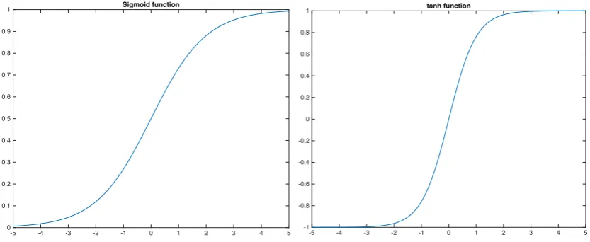
Additionally, there are two commonly used activation functions for non-linear transformation of neural networks, namely the sigmoid function (defined as Equa-tion 2.3) and hyperbolic tangent funcEqua-tion (defined as EquaEqua-tion 2.4). The output ranges of these two activation functions are [0, 1] and [ 1, 1], respectively. Fig-ure 2.2 shows the plots of sigmoid function and hyperbolic tangent function. In this dissertation, the sigmoid activation function is employed in most of the experiments in order to be consistent with methods shown in [54, 55].

f(z) = 1

1 +e z, (2.3)

f(z) = tanh (z) = e

z _e z

-5 -4 -3 -2 -1 0 1 2 3 4 5 0

0.1 0.2 0.3 0.4 0.5 0.6 0.7 0.8 0.9

1 Sigmoid function

-5 -4 -3 -2 -1 0 1 2 3 4 5

-1 -0.8 -0.6 -0.4 -0.2 0 0.2 0.4 0.6 0.8

1 tanh function

Figure 2.2: Plots of sigmoid function and tanh function.

while keep using non-linear activation function (such as the sigmoid function) for hidden layers. Implementing auto-encoders with linear decoder allows us to train networks on real-valued input data without considering strategies to scale examples to a certain range.

Additionally, according to [58], when non-linear activation functions of auto-encoder are changed to linear ones for both auto-encoder and decoder, the auto-auto-encoder will learn essentially the same representation as the Principal Component Analysis (PCA).

2.1.3

Back-propagation

The back-propagation is a common technique to train a neural network applied in conjunction with an optimization method. It attempts to minimize the loss function by calculating the gradient of the loss function with respect to all the weights in the network and then feeding the gradient to the chosen optimization method.

Based on the single-hidden-layer auto-encoder introduced above, the parameters

✓={✓1,✓2}of this model are required to be optimized to minimize the

2.1 Auto-Encoders 15

J(✓) = 1

2kxˆ xk

2

. (2.5)

In addition, a regularization term, also called weight decay term, is added to the cost function so as to prevent overfitting. The regularization term helps decrease the magnitude of the weights. Therefore, the overall cost function for a traditional auto-encoder is described as:

J(✓) = 1 2m

m

X

i=1

kxˆi xik2+

2 kW1k

2

+_kW2k2 , (2.6)

where, xi and ˆxi correspond to the ith training sample and its reconstructed fea-ture, respectively. Furthermore, m is the total number of training samples and represents the weight decay parameter which controls the relative importance of the two terms of the cost function.

In order to train the neural networks, random initialization of W and b is necessary and significant. As asserted in [57], the initialization with identical values for all parameters will result in all hidden layer units of neural networks learning the same function of the input. Thus, in practice, one e↵ective strategy for random initialization is to randomly select values for parameters uniformly in the range [ ",+"], where " represents a value near zero. A good choice to assign " for symmetry breaking is:

"=

p

6

p

Nin+Nout

, (2.7)

where Nin and Nout stand for the number of units in the adjacent layers to ✓. After knowing the structure of the auto-encoder neural network, the forward-pass computation, the objective function applied to training the network, and the initialization strategy for all parameters, the back-propagation learning algorithm can be employed to train the network by optimizing all the weights and bias. Back-propagation is a common approach to train artificial neural networks applied in conjunction with an optimization method. With respect to all the parameters of the network, it computes the gradient of the cost function which will be then fed to the optimization method to update the weights and attempt to minimize the cost function eventually [60]. In order to calculate the gradient of the cost function, a known, desired output value for each input is required.

W :=W ↵ @

@WJ(✓), (2.8)

b :=b ↵@

@bJ(✓). (2.9)

where ↵ is the ratio that a↵ects the quality and speed of learning, which is called

the learning rate. Training is faster when learning rate is large, while it is slower

but more accurate when learning rate is small.

The partial derivatives of the overall cost functionJ(✓), defined in Equation 2.6, can be computed by back-propagation as:

@

@WJ(✓) =

" 1 m m X i=1 @

@WJ(✓;xi,xˆi)

#

+ W, (2.10)

@

@bJ(✓) =

1 m m X i=1 @

@bJ(✓;xi,xˆi). (2.11)

The procedure of back-propagation training algorithm can be divided into two phases: propagation and weight update. The intuition behind back-propagation is as follows. Given an input training examplexand its target output (target output of auto-encoder is the same to the input), the forward propagation starting from the input layer is the first run to generate all the activations of the networks, including the hypothesis output ˆx. Then, the ‘error term’ for each node in each layer is computed backward from the output layer, which measures how much each node was ‘responsible’ for the errors occurred in the output. The error term for nodes in output layer can be directly measured by the di↵erence between hypothesis output and the target output. Based on computed , partial derivatives are calculated for all parameters.

Concretely, the back-propagation algorithm can be described as below:

1. Implement the forward pass, compute activations for all layers from input layer.

2. For output layer (Layer nl), define nl as:

nl ₌ @ @znl

1

2kxˆ xk

2

= (x anl_)· 0_(znl_{), (2.12)}

where, znl denotes the total weighted sum of inputs to Layer n

2.1 Auto-Encoders 17

In this dissertation, we apply sigmoid function as activation function. Thus, the derivative of activation function is 0(znl_{) =a}nl_{(1 a}nl_).

3. For l =nl 1, nl 2, . . . ,2, define l as:

l₌⇣ _Wl T (l+1)⌘_· 0 _zl _{, (2.13)}

4. Compute the partial derivatives (denoted as _r) for parameters:

rWlJ(✓) =

(l+1) _al T_{, (2.14)}

rblJ(✓) =

(l+1)_{. (2.15)}

Then, with the partial derivatives, all parameters can be updated simultane-ously to reduce the cost functionJ(✓) by repeatedly taking steps of gradient descent (use Equation 2.8 and Equation 2.9).

2.1.4

Optimization Algorithms

Gradient descent optimization method has been applied to a variety of computer vision areas to train feature learning algorithms which achieve state-of-the-art per-formance, such as object and scene recognition [39], action recognition [35], content-based image retrieval [61], etc. For instance, Limited-memory BFGS (L-BFGS) and Stochastic Gradient Descent (SGD) are two commonly employed gradient descent methods for optimization. Only brief background knowledge about these opti-mization methods will be included in this section since the implementation details behind these methods are beyond the scope of this dissertation.

SGD makes use of a small randomly-selected subset of training data to ap-proximately estimate the gradient of the cost function in each iteration. Updating parameters in an online fashion, SGD learning framework is attractive because it of-ten requires much less training time in practice than batch training algorithms [63]. The number of training samples used for gradient approximation in each update iteration is called batch size. When the algorithm sweeps through the whole train-ing set, it performs the update for all traintrain-ing samples as Equation 2.8 and Equa-tion 2.9. After each pass, the training data can be shu✏ed to prevent cycles and several passes can be made till the algorithm converges. The appropriate batch size should be determined through experiments to lead the algorithm to converge smoothly. Furthermore, the value of learning rate↵can also significantly influence the convergence of training.

According to [64], the current predominant optimization method in training deep learning is SGD due to its ease of implementation and computational efficiency of training on the large-scale dataset. While it has been adopted extensively in machine learning, SGD has several disadvantages. One major disadvantage is that using SGD optimization algorithm requires much manual tuning or selection of parameters such as learning rate, batch size, and convergence criteria. It is hard to select good parameter values for people especially when they are not familiar with the tasks at hand. On the contrary, L-BFGS, a batch method using a line search procedure, is much more stable to train and easier to check convergence. Whereas, compared with SGD, L-BFGS computes the gradient of the cost function based on the entire training set in each iteration, which makes it not scale gracefully with the large-scale training set. In this dissertation, both gradient methods are applied to optimize di↵erent kinds of neural networks.

2.2

Classifiers

Classification is the problem that identifies a new test sample to one of several pre-defined categories. In this section, several widely used classifiers related to experi-ments of this dissertation will be introduced, which are Softmax regression model, K-Nearest Neighbors algorithm (KNN), and Support Vector Machines (SVM).

2.2.1

Softmax

2.2 Classifiers 19

and continuous data, including multinomial logistic regression [65], multi-class lin-ear discriminant analysis [66], naive Bayes classifiers [67], and artificial neural net-works [39]. Softmax regression is a supervised learning algorithm and is usually implemented at the final layer of neural networks as a classifier to produce the probability distribution over all pre-defined categories.

Regarding the logistic regression, it is a binary classification model. Given a training set: x(1)_{, y}(1) _{, x}(2)_{, y}(2) _{, . . . , x}(m)_{, y}(m) _{with m labeled examples,}

wherey(i)_{2{0,1}represents the label for each example, the hypothesis of logistic}

regression with respect to the model parameters ✓ is:

h✓(x) = 1

1 +e ✓T_x, (2.16)

where model parameters✓are trained through an optimization algorithm (L-BFGS or SGD) to minimize the cost function defined below:

J(✓) = 1

m

" _m X

i=1

y(i)logh✓ x(i) + 1 y(i) log 1 h✓ x(i)

#

. (2.17)

While in softmax regression model, multi-class classification rather than only binary classification is carried on, which means the class label y(i) _{of training}

ex-amples can take more than two values, i.e. y(i) _{2 {1,2, . . . , k}. Thus, for a new}

test example, the model will output the hypothesis that is a k dimensional vector, each value of which represents the probability of test example to belong to the corresponding category. The probability for each class is denoted as: p(y =j|x), for each value of j = 1,2, . . . , k. Concretely, the hypothesis of softmax regression takes the form:

h✓ x(i) =

2 6 6 6 6 4

p y(i)_{= 1|x}(i)_;✓

p y(i)_{= 2|x}(i)_;✓

...

p y(i) _=k|x(i)_;✓

3 7 7 7 7 5= 1 k P j=1

e✓Tjx(i) 2 6 6 6 6 4

e✓T

1x(i)

e✓T

2x(i) ...

e✓T kx(i)

3 7 7 7 7

5, (2.18)

where the term _Pk 1 j=1

e✓jTx(i)

is the normalization term to make the distribution sum

to 1. In addition, ✓1,✓2, . . . ,✓k are the parameters of the softmax model.

As demonstrated in [68], the softmax model is over-parameterized, which means multiple parameter settings can give rise to exactly the same hypothesis function

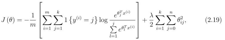
to penalize the parameters with large values. Therefore, based on the hypothesis vector, we can describe the cost function of softmax regression. In the following cost function, an indicator function is defined as 1{·} to depict whether the statement in the function is true, namely 1_{a true statement_} = 1 and 1_{a false statement_} = 0. Thus, the cost function is as follows:

J(✓) = 1

m 2 6 6 6 4 m X i=1 k X j=1

1 y(i) =j log e

✓T jx(i)

j

P

l=1

e✓T lx(i)

3 7 7 7

5+ 2

k X i=1 n X j=0

✓2_ij, (2.19)

where the second term is called weight decay term (also called regularization term), which tends to decrease the magnitude of the model weights and helps prevent overfitting.

With the cost function J(✓) shown above, softmax regression is now strictly convex, which can guarantee only one unique solution is trained. In order to make use of gradient descent optimization method, the derivatives (denoted as_r✓jJ(✓))

of cost function with respect to all parameters ✓ are required:

r✓jJ(✓) =

1 m m X i=1 ⇥

x(i) 1 y(i)=j p y(i) =j_|x(i);✓ ⇤+ ✓j. (2.20)

2.2.2

K-Nearest Neighbors

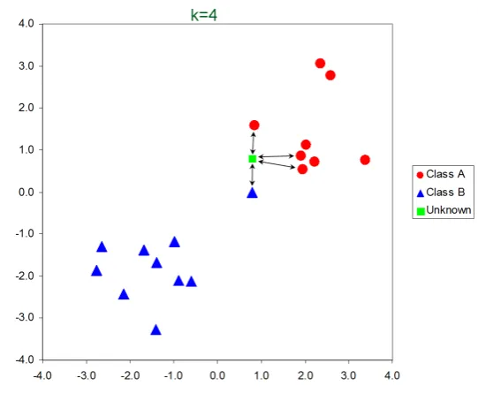
The K-Nearest Neighbors (KNN) algorithm [69] is one of the oldest and simplest methods for pattern recognition. Nevertheless, it usually has competitive perfor-mance or achieves state-of-the-art in some domains when incorporated cleverly with the prior knowledge [70]. The input of KNN algorithm is training examples in the feature space with corresponding labels. The output for KNN applied to classification tasks is the class name for the unlabeled test (or query) example. The Figure 2.3 shows a sample plot of KNN criteria.

Given the training set features with labels, Y = _{y1, y2, . . . , ym}, which con-tains m examples, and a query example x. The descriptors for query and training examples are in the same feature space. Thus, thek⇤_{-th nearest neighbor, denoted}

asNk(x), ofx in Y is defined as:

Nk⇤(x) =k⇤arg min

2.2 Classifiers 21

Figure 2.3: Sample plot of K-Nearest Neighbors criteria where k = 4 and the training examples have two di↵erent labels, ‘Class A’ and ‘Class B’.

where functiond(x, yi) represents the distance between queryxand training exam-ple yi. A commonly used distance metric for KNN classifier is Euclidean distance [71]. The resulting k nearest neighbors is Nk(x) = {N1⇤(x), N₂⇤(x), . . . , N_k⇤(x)}.

After the indexing/ranking system generates a set of k nearest neighbors hy-potheses for each query sample, the voting criteria should be selected to leverage the KNN retrieval list so as to yield the final label for each query example. The parameter k is a positive integer. When k= 1, the KNN algorithm simply assigns the class of the single nearest neighbor to query.

There are several possible voting criteria which exploit the information provided by the ranks of nearest neighbors and their corresponding distances to the query descriptors. The commonly employed criteria are as follows:

• Majority Vote: It counts the total number of votes for each query examples

without taking into account the rank and distance information. The query example is assigned to the class that appears most common among its k

nearest neighbors.

• Rank Vote: It exploits the rank information of retrieval list independently of

distance information.

• Distance Vote: It uses the absolute distance information of obtained nearest

• Distance Ratio Criteria: [72] It assigns a weight computed by distance ratio to the contributions of neighbors in order to discard unreliable votes. The weight for each nearest neighbor is defined as: 1_d, where d is the distance between the query and the neighbor.

• Adaptive Criteria: [73] The weights of nearest neighbors are derived from the

distance. Given a ranking list containing k nearest neighbors, the weight (denoted as (x, y)) of a certain neighborywith respect to queryxis defined by:

(x, y) = max (d(x, Nk⇤(x)) d(x, y),0), (2.22)

whered(x, y) is the distance between queryxand a certain nearest neighbor

y. This criteria asserted by authors is more comparable across queries than the absolute distance d(x, y) and the distance ratio criteria in many cases.

Weighting method is beneficial to KNN algorithm because it guarantees the nearer neighbor contribute more than the more distant ones. Hence, for a query example, the final voting class is the one with the highest weight in the ranking list. In this dissertation, we adopt the adjusted version of Adaptive Criteria. We mea-sure the weight (x, y) based on the distance from query to the reference (k⇤+ 1)-th nearest neighbor whenk⇤ < m, wheremis the total number of examples in training set. While when k⇤ = m, the criteria are the same as [73]. The reason why this adjustment is applied is because whenk⇤ _{< m, the weight ofk}⇤_{-th nearest neighbor}

is zero that means it will contribute nothing to the final voting. Thus, the final voting will only depend on the weights of (k⇤ _{1) nearest neighbors, which results}

in the loss of k⇤_{-th nearest neighbor’s information of ranking list. Moreover, this}

adjustment also fixes the potential problem of no voting is yielded when k = 1. Therefore, in this dissertation, when the value ofk⇤ _{is less than m, a retrieval list}

consisting of (k⇤+ 1) nearest neighbors is fed to KNN algorithm and the applied voting criteria is:

(x, y) = max (d(x, Nk⇤₊₁(x)) d(x, y),0). (2.23)

2.2.3

Support Vector Machines

2.2 Classifiers 23

support vector machines along with neural networks are now playing significant roles as the standard tools for machine learning and data mining [74].

As stated in [26], SVM is a learning machine for two-group classification prob-lems, which conceptually implements the ideas to map the input data into some higher dimensional feature space through some non-linear mapping methods. Fol-lowing that, a linear optimal decision surface will be constructed in this feature space with special attributes that ensure the high generalization capacity of the network. Unlike traditional methods that aim to minimize the training error, the goal of SVM is to minimize the upper bound of generalization error by maximizing the margin between the separating data [75].

Since the dimension of the feature space is huge, how to find the hyperplane that can separate the two classes data well is the main problem. However, according to [26], in order to construct the optimal hyper-plane separating data into two classes, only a small amount of training data needs to be taken into account, namely the support vectors, which can determine the margin between two-group data. It is the properties such as condensing training data information and providing the sparse representation with only very small number of data points that makes the support vector machine attractive and popular [76].

As demonstrated in [26, 77, 78], given a set a labeled training data contain-ing m examples, x(1)_{, y}(1) _{, x}(2)_{, y}(2) _{, . . . , x}(m)_{, y}(m) _{, where y}(i) _{2 { 1,1}}

represents the label for each example, the goal for SVM is to find the maximum margin hyperplane that separates the points withy(i) _{= 1 from those points having}

y(i) _{= 1.}

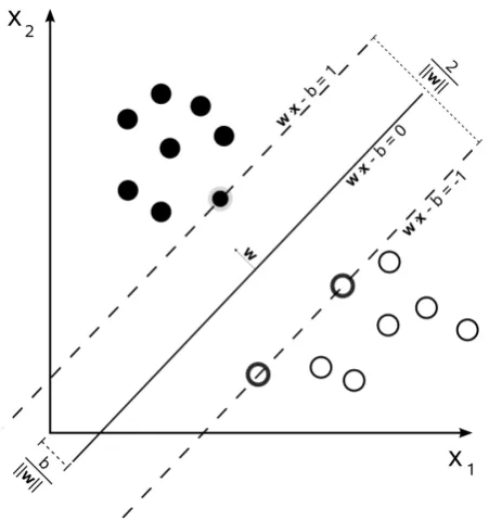
The input data points are said to be linearly separable when there exists a vector w and a scalar b so that the two hyperplanes described by two equations below can separate the input data and there are no points lie between them. The region bounded by them is called ‘margin’.

w·x(i) b= 1, (2.24)

w·x(i) b= 1, (2.25)

Based on geometry, it can be found that the distance between these two hy-perplanes is 2

kwk. In order to maximize the width of margin, kwk should be

Figure 2.4: An example of linear separating hyperplane for the separable case in 2-dimensional space. The maximum margin distance is shown. The support vectors are those dots and circles, which define the margin of maximum separation between two classes.

y(i) w·x(i) b 1, i= 1,2, . . . , m. (2.26)

Thus, the optimal hyperplane defined below is the unique one that can separate the training data points with a maximal margin, where w0 and b0 are parameters

to depict the optimal hyperplane:

w0·x b0 = 0. (2.27)

It determines the direction _|w_w| where the distance between two di↵erent classes of training vectors is maximal. The distance can be represented by:

⇢(w, b) = min

(x:y=1)

x·w

|w_| (xmax:y= 1)

x·w

|w_| . (2.28)

The hyperplane (w0, b0) is the argument that makes the distance maximal:

⇢(w0, b0) =

2

|w0|

= _p 2

w0·w0

. (2.29)

Therefore, it can be seen that constructing the optimal hyperplane by minimizing

2.2 Classifiers 25

When there exists no hyperplane to split the two-classes examples without error, the soft margin method will be used to choose a hyperplane which separates the training data as cleanly as possible, namely with a minimal number of errors, while still maximize the distance to the nearest split examples [26,79]. To solve this kind of problems, some non-negative variables ⇠i 0,for i = 1,2, . . . , m is introduced, which measures the degree of misclassification of the training data x(i)_{. The new}

constraint is:

y(i) w· x(i) b 1 ⇠i, i= 1,2, . . . , m. (2.30)

Subjected to this constraint, the objective function for constructing an optimal separating hyperplane can be expressed as:

min w,b,⇠

(

1 2kwk

2

+C

m

X

i=1

⇠i

)

, (2.31)

where x(i) _{is a function mapping the datax}(i) _{to higher-dimensional space, and}

C >0 is the regularization term.

The original hyperplane algorithm for SVM is a linear classifier in the parameter space. Whereas, SVM is easily extended to a non-linear classifier by applying the kernel trick . Through choosing a proper mapping , the training points could become linearly or mostly linearly separable in the high-dimensional feature space. Figure 2.5 intuitively shows how kernel machine works. The resulting algorithm in the feature space is formally similar to the algorithm introduced before, except that every dot product is replaced by a nonlinear kernel function, which allows the maximum-margin hyperplane to be constructed in the transformed feature space. Since this transformation may be not linear, the resulting hyperplane in high-dimensional space could be non-linear in the original input space.

Figure 2.5: Kernel machines used to compute a non-linearly separable function into a higher dimension linearly separable function.

2.3

Stacked Auto-Encoders and Greedy

Layer-wise Training

Deep learning approaches attempt to learn complex feature hierarchies. Lower-level features are first learned and used as the input to learn features at higher-levels. A system with the capacity to learn multi-level feature representations automatically can yield complex transformation functions that map the input data directly to higher-level abstract representations without heavily requiring hand-engineered features [82]. This kind of automatic learning is crucial especially when people do not have much prior knowledge on how to explicitly describe the raw input data. It becomes increasingly significant as the amount of accessible sensory data and the range of applications of machine learning continuing growing.

2.3 Stacked Auto-Encoders and Greedy Layer-wise Training 27

global fine-tuning of model’s parameters is performed using a supervised training criterion.

The greedy layer-wise pre-training approach has been shown empirically to help to mitigate the difficult optimization problem of deep networks, which prevents the training from getting stuck in the kind of poor solutions that previous work with random initializations typically reaches [83]. Discussion in [82] shows that unsu-pervised training amounts to a form of regularizer or prior for the deep network, which constrains a region in parameter space where a solution is allowed. The constrained region is near to the features learned by unsupervised training which hopefully will capture the important statistical structure of input data. There are three aspects particularly significant in the greedy layer-wise training strategy [48]:

• Pre-training one layer at a time in a greedy way,

• Leveraging unsupervised learning algorithm at each layer so as to preserve the information from input,

• Performing global fine-tuning over the entire neural network with respect to training criterion of interest.

Therefore, the training procedure of SAE is based on the training of each build-ing block, such as Auto-Encoder and Softmax classifier discussed above:

1. Unsupervised Training: Given input data, train the first auto-encoder to

learn hidden layer features and also the initial values for network parameters

✓={W, b}.

2. Unsupervised Training: The hidden layer features from the first auto-encoder

are fed to another auto-encoder as the input. Train the second auto-encoder to obtain corresponding hidden layer features and weight parameters.

3. Repeat training process as in step (2) until the desired number of additional layers are trained.

4. Supervised Training: Feed the hidden layer features of the last auto-encoder

to a supervised classifier, such as Softmax model, to pre-initialize the weights for classifier.

5. Supervised Training: Implement a global fine-tuning on the entire network

2.4

Convolutional Neural Networks

According to [42], though it is found to be difficult to train deep supervised neural networks before greedy layer-wise unsupervised pre-training is used, there is one notable exception in artificial neural networks: Convolutional Neural Networks (CNN), which are inspired by the hierarchy of the visual system. The first compu-tational, multilayered neural network model is found in Neocognitron proposed by Fukushima [85], which is based on the local connectivities between neurons and hi-erarchically organized transformations of images. Later, following this idea, LeCun and his collaborators built and trained gradient-based convolutional networks and set state-of-the-art on several pattern recognition tasks [37]. To this day, convolu-tional neural networks hold state-of-the-art performance in various computer vision areas, such as object recognition [49], face recognition [86], image classification [39], image parsing [87], etc.

Convolutional neural networks are deep hierarchies composed of several convo-lutional layers, each of which is often followed by a subsampling layer, and one or more fully connected layers the same as in a standard multi-layer neural network. The architecture of CNN is designed to leverage the 2D structure of input images or other types of 2D input data. A convolutional neural network automatically provides some degree of translation invariance which is achieved by local connec-tions and tied weights following with some form of pooling operaconnec-tions [88]. Another advantage of CNNs compared with standard deep neural networks is the ease of training because CNN has much fewer parameters to be optimized, especially when applying on high-resolution images, than fully connected networks with the same number of hidden layers. For fully connected networks, it is computationally ex-pensive to learn features from the entire image. Regarding convolutional networks, due to the local connectivity property between neurons, CNNs allow each hidden unit to connect to only a small subset of the input units. Specifically, each hidden unit of the locally connected network, such as CNN, will only connect to pixels in a small contiguous region in the input image [42]. Furthermore, based on the weight sharing idea, each filter is replicated across the entire visual field, which means the replicated units share the same weight vectors and bias to form a new feature map. Thus, the learning efficiency can be increased using weight sharing by significantly reducing the number of free parameters to be learned [59].