This is a repository copy of Almost separable matrices.
White Rose Research Online URL for this paper:
http://eprints.whiterose.ac.uk/147160/
Version: Accepted Version
Article:
Aldridge, M orcid.org/0000-0002-9347-1586, Baldassini, L and Gunderson, K (2017)
Almost separable matrices. Journal of Combinatorial Optimization, 33 (1). pp. 215-236.
ISSN 1382-6905
https://doi.org/10.1007/s10878-015-9951-1
© Springer Science+Business Media New York 2015. This is an author produced version
of a paper published in Journal of Combinatorial Optimization. Uploaded in accordance
with the publisher's self-archiving policy.
Reuse
Items deposited in White Rose Research Online are protected by copyright, with all rights reserved unless indicated otherwise. They may be downloaded and/or printed for private study, or other acts as permitted by national copyright laws. The publisher or other rights holders may allow further reproduction and re-use of the full text version. This is indicated by the licence information on the White Rose Research Online record for the item.
Takedown
If you consider content in White Rose Research Online to be in breach of UK law, please notify us by
Almost Separable Matrices
Matthew Aldridge
∗1, Leonardo Baldassini
†2and Karen
Gunderson
‡11
Heilbronn Institute for Mathematics Research, School of
Mathematics, University of Bristol, Bristol, UK
2
School of Mathematics, University of Bristol, Bristol, UK
July 26, 2018
Abstract
An m×n matrixA with column supports {Si}is k-separable if the disjunctionsSi∈KSiare all distinct over all setsKof cardinalityk. While
a simple counting bound shows thatm > klog2n/krows are required for a separable matrix to exist, in fact it is necessary for m to be about a factor ofkmore than this. In this paper, we consider a weaker definition of ‘almostk-separability’, which requires that the disjunctions are ‘mostly distinct’. We show using a random construction that these matrices exist withm =O(klogn) rows, which is optimal for k = O(n1−β). Further,
by calculating explicit constants, we show how almost separable matrices give new bounds on the rate of nonadaptive group testing.
1
Introduction
LetA∈ {0,1}m×n be anm×nbinary matrix, and writeSi for the support of itsith column (that is, the locations of the1s). ThenAis said to bek-separable if the setsS
i∈KSi are all distinct over all setsK ∈ {1,2, . . . , n}of cardinality k (see Definition 1, to come).
Separable matrices were first introduced by Erd˝os and Moser in 1970 [9] and have since been studied in different contexts, including coding theory, combina-torics and, as we discuss later, group testing, where they play a very important role.
Separable matrices are often studied through the slightly stronger concept of disjunct matrices(see Definition 3). Disjunct matrices were first introduced by Kautz and Singleton [11] and, just like separable matrices, they have been extensively studied in coding theory, combinatorics and group testing [5, 7, 8, 10, 18].
A central question in the study of both separable and disjunct matrices is the following: Given n and k, how large must m be for there to exist either
an m×n k-separable or disjunct matrix? In this paper, we investigate the asymptotics for separability asn→ ∞, wherek may grow withn.
A simple counting bound (Theorem 2) shows that m ≥Ω(klogn/k) rows are required. Disappointingly, when k =o(n) this bound is not tight, and we require roughly a factor ofkmore than this, as in fact it has been shown [7, 5] that m ≥ Ω(k2logn/logk) is needed. This lower bound is motivated by the
connection between disjunctness and separability, as we discuss in Section 2. Notice that when k grows linearly with n, taking the identity matrix is order optimal – for this reason, we consider onlyk=o(n) in this paper.
In order to meet the lower boundm≥Ω(klogn/k), we consider a relaxation of the requirement ofk-separability toalmostk-separability. Roughly speaking, a matrix is almost k-separable if the sets S
i∈KSi are ‘usually’ distinct – see Definition 4 for a formal definition.
Our main result shows that it is possible to achieve almost separability with onlyO(klogn) rows (Theorem 7). Whenk=O(n1−β), for anyβ ∈(0,1], this is order-optimal to the counting bound. However, we also aim to get best possible constants for m - a goal motivated by the study of the rate of group testing algorithms.
Group testing is an old and well-studied search problem, first considered by Dorfman [6], where the goal is to recover a sparse subset ofkdefectiveelements spread amongn otherwise identical items. Instead of testing each item for de-fectiveness individually, classic group testing algorithms test items in batches. In the noiseless binary model we consider, tests can only reveal whether a given set contains at least one defective (a positive test) or no defectives (a negative test). The connection between separable matrices and nonadaptive group test-ing is well-known, and we discuss it in Section 5. For the moment, we just observe that a sequence of tests designed a priori (nonadaptive group testing) has a natural binary-matrix representation: each length-nrow represents a test, with entries being1if the corresponding item is being included in the test.
A matrix beingk-separable is equivalent to having zero probability of error for nonadaptive group testing, while a matrix being almostk-separable is equiv-alent to having a small probability of error. The ‘arbitrarily small probability of error’ criterion we consider here is the same as that in Shannon’s theory of channel coding.
With this comparison in mind, we consider the concept of rate of group testing (Definition 10) for k = n1−β defective items in a population of size n, which can be thought of as the amount of information conveyed by each test. Using a separable matrix with m = Ω(k2logn/logk) rows leads to a
group testing rate of 0. However, using an almost separable matrix with m= O(klogn) rows gives a strictly positive rate, with the rate depending on the contant implied by the big-O. Hence, here we are interested in getting good constants form, not only in order-wise results.
2
Separable matrices
We begin by recalling the definition of a separable matrix.
Definition 1. Given anm×nbinary matrix A= (aij)∈ {0,1}m×n, we shall write Si :={j :aij =1} for thesupport of columniand for K ⊆ {1,2, . . . , n} also writeS(K) :=S
i∈KSi for the support of a disjunction of columns. The matrixAis calledk-separablematrix if the for all setsKof sizek, there is no other setL also of sizekwithS(L) = S(K).
The casek = 0 is trivial, so we assume k ≥ 1 throughout. We shall also assumek≤n/2, which will be no restriction in the limiting regimes we study.
The following counting bound is described by Chen and Hwang as “simple-minded” [5].
Theorem 2. Let M(n, k) be the smallest m such that an m×n k-separable matrix exists. Then
M(n, k)≥log2
n
k
.
Proof. Clearly
|{S(K) :|K|=k}| ≤ |P({1,2, . . . , m})|= 2m,
where P denotes the power set. Hence for A to be k-separable we require 2m≥ n
k
, and taking logarithms gives the result.
Using the lower bound of
n k
k ≤
n
k
≤enkk (1)
(which we shall use many times in this paper), we see that ak-separable matrix must have at leastm≥klog2n/k= Ω(klogn/k) rows.
As we anticipated, separable matrices are tightly related to another class of matrices, namely that of disjunct matrices.
Definition 3. With the notation of Definition 1,Ais k-disjunct if for all sets K of cardinality|K|=k, there does not existi6∈ K such thatSi⊆S(K).
In the language of set systems, a matrix Abeing k-seperable is equivalent to the family {Si}ni=1 being k-union-free, and A being k-disjunct is equivalent
to{Si}ni=1 beingk-cover-free.
It’s easy to see thatk-disjunctness impliesk-separability (see, for example, [11], [7, Section 7.2], or the special case ǫ = 0 of Lemma 6 below). On the other hand, Chen and Hwang [5, Theorem 2] have shown that it is possible to construct a k-disjunct matrix from a 2k-separable matrix by adding at most one row to it, which means that disjunct and separable matrices share the same order-wise asymptotics. Dyachkov and Rykov have quantified these asymptotics by showing thatm≥Ω(k2logn/logk) rows are necessary for a matrix to be
As disjunctness is a stronger (and, in some ways, simpler) property than separability, efforts to derive upper bounds on m for separable matrices have often proceeded via the construction of disjunct matrices. In their seminal paper [11], Kautz and Singleton give a probabilistic existence theorem for k-disjunct matrices withm=O(k2logn) rows. In the group testing literature there exist
explicit constructions of testing schemes withO(k2logn) rows, see for example
Porat and Rothschild [17].
3
Almost separable matrices
Since separable matrices cannot meet the counting bound, it would be of interest if a matrix could be close to being separable using onlyO(klogn) rows. Such a matrix would be order-optimal.
With this in mind, we define the concept of analmost separable matrix in a similar manner to Defintion 1.
Definition 4. With the notation of Definition 1, A ∈ {0,1}m×n is ǫ-almost k-separable if for at mostǫ nk
setsKof sizekdoes there exist another setLof size kwithS(L) =S(K).
An analogous definition is present in for example [22], where almost separable matrices are calledweakly separating designs. Note that settingǫ= 0 gives the definition of a separable matrix.
The main result of this paper is to show the existence ofǫ-almostk-separable matrices with m = O(klogn) rows (see Theorem 7 below). We also examine the implicit constants for the case whenk=n1−β grows polynomially inn.
Malyutov [14] effectively showed that ǫ-almost k-separable matrices exist withm= (k+o(1)) log2nrows in the regime wherekis fixed asn→ ∞. This
is a special case of a more general result Malyutov proved using an information theoretic argument – this and similar work is reviewed in [15]. Seb˝o showed effectively the same result [19], again for fixedk, by analysing a concrete bound on the probability that there are two different sets of size kwhose disjunctions coincide – we follow a similar route here later. The same result fork fixed and n→ ∞was rediscovered by Zhigljavsky [22, Theorem 5.5]. Although technically different from Seb˝o’s argument, Zhigljavsky’s proof is morally similar: given two setsKandLofkcolumns each, Zhigljavsky counts how many rows it is possible to construct that would produce the same value for both S(K) andS(L). He calls this number a R´enyi coefficient and only considers designs with fixed- or bounded-size tests.
Our result improves on these by allowingkto vary arbitrarily withn, subject to k = o(n). In our discussion of group testing in Section 5 we show how, in some regimes, this work also improves on recent results on nonadaptive group testing giving bounds of the formm=O(klogn).
The definition of a disjunct matrix (Defintion 3) can similarly be weakened to give an almost disjunct matrix. (This definition also appears in [16] and, previously, in [12].)
Definition 5. With the notation of Definition 1,Aisǫ-almostk-disjunct if for at mostǫ nk
Note again that ǫ = 0 corresponds to a disjunct matrix. Unsurprisingly, almost disjunctness implies almost separability.
Lemma 6. Let A be an ǫ-almost k-disjunct matrix. Then A is ǫ-almost k -separable (with the sameǫ andk).
Proof. We prove the contrapositive. Suppose A is not ǫ-almost k-separable. Then there are more than ǫ nk
sets of sizek breaking separability. Let K be one of these sets, so there is another setLof sizekwithS(K) =S(L). Letting i ∈ K \ L, we have Si ⊆ S(K), breaking disjunctness. Hence there are more thanǫ nk
sets breaking disjunctness, andAis notǫ-almostk-disjunct.
Mazumdar [16] shows that there exist almostk-disjunct matrices withm= O(k3/2√logn) rows in the regime k ∼ nδ, δ > 0, which is the same as that we consider for group testing. Mazumdar’s construction is similar to those of Kautz and Singleton [11] and Porat and Rothschild [17]. In particular, [11] shows how to build fully disjunct matrices withO(k2log2
klognn) rows by mapping the symbols of aq-ary Reed-Solomon code to unit-weight binary vectors of length q, while [17] improves on this scheme by replacing the RS code with a linear q-ary code achieving the Gilbert-Varshamov bound. This produces fully disjunct matrices withO(k2logn) rows. This improves on the Ω(k2logn/logk) required
for full disjunctness or separability, while being less good than the O(klogn) we achieve for almost separability here.
Our main result is then the following.
Theorem 7. For any sequence k = k(n) = o(n) and ǫ > 0, there exist an
ǫ-almostk-separable matrix withm=O(klogn)rows. More precisely, forα∈[ln 2,1], define
M1(n, k, α) = 1
−ln(1−2e−α+ 2e−2α)kln n k,
M2(n, k, α) =
1
−ln(1−2e−α+ 2e−α(1+1/k))lnnk, (2)
M(n, k) = min
α∈[ln 2,1]max{M1(n, k, α), M2(n, k, α)}.
Then for any ǫ, δ >0, for n sufficiently large, and m >(1 +δ)M(n, k), there exists andm×n ǫ-almostk-separable matrix.
Consider the special caseα= ln 2. It is possible to see thatM2 dominates,
and hence that there exist almost separable matrices withm= (1 +δ)klog2nk
rows. Note that this is sufficient to show them=O(klogn) result – and comes with a slightly easier proof than the general case (see below). This bound also meets the Malyutov–Seb˝o result ofm∼klog2nfork constant. However, it is
possible to get slightly better constants for mostk=k(n) by allowing different values ofα. In particular,M2withα= 1 gives the best result in many regimes.
In Section 5 we discuss the constants in more detail in the regimek=n1−β forβ∈(0,1). (The reader may wish to skip ahead to Figure 1, to get a feeling for this result.)
4
Proof of main result
We proceed to prove Theorem 7 as follows. Fix n and k. We will choose A
to be an m×n matrix (where m will be determined later) with each entry independently1with probability pand0with probabilityq= 1−p, for some palso to be chosen later. We aim to show that there is a choice ofm andpso that, with positive probability, Ais ǫ-almost k-separable, and hence that such a matrix exists.
The following bound will be important, and is fairly well known – see for example Seb˝o [19], who analyses its asymptotics for fixedkasn→ ∞.
Lemma 8. Let A be a randomly chosen matrix in {0,1}m×n with each entry
independently1 with probabilityp. For any setK of size k≤n/2, then
P(∃ L with|L|=k, S(L) =S(K))≤ k−1
X
b=0
k
b
n
−k k−b
1−2qk+ 2q2k−bm .
(3)
Proof. Say that an overlap occurs if there exists L with |L| =k and S(L) = S(K). Take two distinct setsK,L, both of sizek, that haveb=|K ∩L|elements in common. Then a rowj ofAcould distinguish betweenKandLin two ways: either we have j ∈ S(K) while j /∈ S(L), or the other way round: j ∈ S(L) whilej /∈S(K).
If the entries of the rowajare IID Bernoulli(p), these two events each occur with probability qk(1−qk−b) = qk −q2k−b. Hence, row j fails to distinguish betweenKand Lwith probability 1−2qk(1−qk−b) = 1−2qk+ 2q2k−b.
Since the rows ofAare IID, the whole matrix fails to distinguish betweenK andL with probability (1−2qk+ 2qk−b)m.
The result then follows by a union bound overL, noting that the number of sets of sizeksharingb elements withK is precisely kb n−k
k−b
.
The main work in this paper is a careful asymptotic analysis of the overlap probability (3), showing for which mit can be made arbitrarily small.
Lemma 9. For every sequence k =k(n) = o(n), ε, δ > 0, there exists n0 so
that if n > n0 and m >(1 +δ)M(n, k), with M(n, k) as in Theorem 7, then
P(overlap)< ε.
Proof. We first prove that it suffices to have m > (1 +δ)M2(n, k,ln 2), with
M2(n, k,ln 2) = (1 +o(1))klog2nk. This is simpler to prove than the full result
and illustrates the main techniques.
Here, we takep= 1−2−1/k, as does Seb˝o [19], so that q= 2−1/k. This is a special case of the general value ofpused in the appendix,p= 1−e−α/k, by takingα= ln 2. Note that, in group testing parlance, this is the value ofpthat gives a 50 : 50 chance of a test being positive. The bound (3) then becomes
P(overlap)≤ k−1
X
b=0
k
b
n
−k k−b
1 22
b/k m
It will be convenient to writec = k−b for the number of nonoverlapping items, to get
P(overlap)≤ k X
c=1
k
k−c
n
−k c
1 22
(k−c)/k m = k X c=1 k c n −k c 2−cm/k.
Whenm >(1 +δ)klog2nk, then the terms in the above sum are decreasing
since k c+1
n−k c+1
2−(c+1)m/k k
c n−k
c
2−cm/k =
(k−c)(n−k−c)2−m/k (c+ 1)2
≤c
2−nc+k(n−k)
nk(c2+ 2c+ 1) (since 2
−m/k
≤1/nk)
≤14,
forn >2kandk≥2. Thus, the probability of an overlap can be estimated by the largest term with
P(overlap)≤k(n−k)2−m/k k X
c=1
1
4 c−1
≤kn2−(1+δ) log2nk4
3
=nk(nk)−1−δ4 3 ≤2(nk)−δ,
which, for fixedδ >0, can be made arbitrarily small fornsufficiently large. Further, since log2nk ≤ 2 log2n, we see that m > (1 + δ)klog2nk =
O(klogn).
We can get the more general result that it suffices to havem >(1+δ)M(n, k), withM(n, k) as in (2), by instead takingp= 1−e−α/k, and then optimising over α. The analysis is very similar to that above, but somewhat more longwinded. The interested reader is directed to the appendix for the details.
Proving our main result is now straightforward.
Proof of Theorem 7. Choose the matrixAat random as above, withm and n chosen as in Lemma 9 so that the overlap probability is at mostǫ/2.
WriteX for the number of setsK of sizekthat experience an overlap. It is clearAwill beǫ-almostk-separable provided thatX≤ǫ nk
. Then we have
P
X > ǫ n
k
≤ 1
ǫ nkEX,
by the Markov inequality. But this expectation is, by Lemma 9
EX= X
|K|=k
P(Khas an overlap) =
n k
Hence, our randomA is ǫ-almost k-separable with probability at least 1/2, so such matrices must exist.
5
Rates for nonadaptive group testing
In this section, we show how the use of almost separable matrices can give new results on the rate of nonadaptive group testing.
As we outlined in the introduction, in a nonadaptive group testing procedure we aim to find a subsetKofkdefective items within a population ofnidentical items. We use mpooled tests. Recall that the outcome of a test j is positive if one or more of the defective items is in the test pool, and negative if none of them are. We summarise our testing procedure by a matrix A= (aij), where aij =1 denotes that itemi is in the pool for test j, andaij =0 denotes that it is not. Recalling the notation of Definition 1, the set of positive tests for a defective setK is preciselyS(K).
The aim is, given the outcomes S(K) and the matrix A, to identify the defective setK. Clearly if there is no other Lwith S(K) =S(L), then we can findK (at least theoretically: for study of practical algorithms for this, see, for example, [1, 4, 20, 13, 21]). Conversely, if there is anLwithS(K) =S(L), then our error probability is at least 1/2.
A comprehensive survey of combinatorial group testing is given in [7]. Like-wise, the study of nondeterministic testing schemes is addressed in the field of probabilistic group testing – see for example [22] and references therein. The derivation of both non-constructive results and practical algorithms has been addressed in different contexts, including combinatorial [7, 14, 16, 19], proba-bilistic [1, 22] and information-theoretic [2, 3, 15, 17, 20] scenarios.
The connection between separable matrices and nonadaptive group testing is well explored. In particular, if there are known to be exactly k defective items, then a testing matrix will allow us to find the defective set with certainty if and only if it is k-separable. The advantages of using what we call almost separability for group testing in the fixed-kregime have also been discussed in [22].
While separable matrices allow detection with zero probability of error, the study of group testing within the scope of information theory and the need for efficient algorithms generated an interest in nonadaptive group testing with low – but not necessarily zero – probability of error, a situation which has gained considerable attention [1, 4, 20, 14, 13, 2, 21]. Here the probability of error is defined as an average over all possible defective sets of sizek; that is,
P(error) = 1n k
X
|K|=k
P(error| K).
Baldassini, Johnson and Aldridge [3] introduced a concept of the rate of group testing to quantify how well a group testing design works. (An earlier definition of rate for the fixedkregime had been introduced by Malyutov [15].) The rate is the ratio of the number of tests to the counting bound log2
n k
Definition 10. Consider a group testing problem withnitems of whichkare defective. A design withmtests is said to haverate R=m/log2 nk
.
Given a sequence of group testing problems for nitems of which k=k(n) are defective, a rate Ris said to be achievable for a designAif, for anyǫ >0, the design finds the defective set with error probability at mostǫ with rate at leastR fornsufficiently large.
We follow Baldassini et al. [3, 1] and study achievable rates in regimes where k=k(n) =n1−β for different values of the sparsity parameter β∈(0,1].
Note from the above that using ak-separable matrix with m≥Ω(k2logn/
logk) tests gives rate 0 for all values ofβ <1.
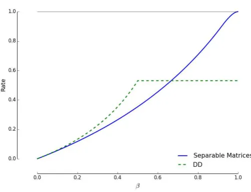
As far as we are aware, the best known rate for nonadaptive group testing until now is achieved by the DDalgorithm of Aldridge, Baldassini and Johnson [1], which has a lower bound on the maximum achievable rate of
RDD(β) = 1 e ln 2min
β
1−β,1
≈0.53 min
β
1−β,1
, (4)
together with the Malytuov–Seb˝o result that R = 1 can be achieved in the fixed-k regime.
Baldassini, Johnson and Aldridge [3] also showed that for adaptive group testing, the generalized binary splitting algorithm of Hwang [7] gives a rate of 1 (the best possible) for allβ∈(0,1].
From Theorem 7, we know that using anǫ-almost k-separating matrix will find the defective set with error probability at mostǫ, since the sets Kwithout overlaps can by definition be recovered with certainty. Hence, the number of rows of the almost separating matrix gives bounds on the rate. Therefore, using our above results, we have the following:
Theorem 11. For β ∈(0,1] and k =n1−β, the maximum achievable rate of
nonadaptive group testing withnitems of whichkare defective is bounded below by
R≥ ln 21 max α∈[ln 2,1]min
2αe−α β
2−β,−ln 1−2e
−α+ 2e−2α
. (5)
Figure 1 illustrates the result of Theorem 11. Note that our result improves over the best known result forβ >2/3, and meets the Malyutov–Seb˝o point as β →1.
Proof. Following directly from Theorem 7 and the definition of rate, we have
R≥ln 21 max α∈[ln 2,1]min
n
−ln1−2e−α+ 2e−α(1+1/k)k β 2−β,
−ln 1−2e−α+ 2e−2αo ,
noting that, whenk=n1−β,
klog2nk=
2−β β klog2
Figure 1: Bounds on rates of group testing, showing the DD bound (4) of Baldassini et al, and our new result Theorem 11.
Whenβ = 1, the second term is the minimum. Whenβ <1, since we have that k→ ∞, we can take limits in the first minimand. We have
−ln 1−2e−α+ 2e−α(1+1/k) k
=−ln1−2e−α+ 2e−αe−α/kk
=−ln
1−2e−α+ 2e−α
1−αk +o 1
k
k
=−ln
1−2e−αα k +o
1 k
k
=
2e−αα k +o
1 k
k
→2αe−α.
The result follows.
Note that our ‘simpler’ result with α= ln 2 gives a bound almost as good the general case, namely
R(ln 2) = β 2−β.
In particular, this choice of α= ln 2 is optimal at β= 1.
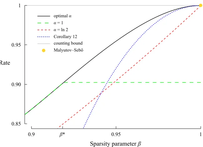
Note also that for all but the sparsest cases, we get the bound by taking α= 1. Specifically, forβ≤β0, where
β0= −2 ln(1−2e
−1+ 2e−2)
optimal α α = 1 α = ln 2 Corollary 12 counting bound Malyutov–Sebő 1
0.95
0.90
0.85
0.9 β* 0.95 1
[image:12.595.135.461.120.356.2]Sparsity parameter β Rate
Figure 2: Bounds on rates of group testing for largeβ, showing Theorem 11 for different values ofαand the approximation of Corollary 12.
the best value of the bound is
R(1) = 1 ln 2min
2e−1 β
2−β,−ln 1−2e
−1+ 2e−2
= 1 ln 22e
−1 β
2−β
≈1.06 β 2−β.
Forβ ∈ (β0,1), the optimal rate is given as the maximum in (5), and the
optimalαis that which achieves the maximum. It’s easy to see forβ ≥β0that
the maximum overαis achieved when the two terms in the minimum are equal, and this is simple to solve numerically. However, here we also provide some closed form approximations to this which could be useful.
Corollary 12. For 2 ln 2
1+ln 2 < β <1andk=n
1−β, the maximum achievable rate
of nonadaptive group testing with nitems, of which k are defective, is bounded from below by
R≥1−ln 21 ln 1 +
2(1−β) ln 2 β(1−ln 2)
2!
This is illustrated in Figure 2. From this, we see that the bound of Corollary 12 is very good forβ≈1, but that whenβis not much aboveβ0, then the bound
of simplyα= 1 is better. Hence, setting
β1=
2 ln 2
and takingβ0as above, we get the following bound:
Corollary 13. For β ∈ (0,1) and k = n1−β, the maximum achievable rate
of nonadaptive group testing with nitems, of which k are defective, is bounded from below by
R≥ 1 ln 2
2e−1 β
2−β if β≤β0
−ln(1−2e−1+ 2e−2) if β
0< β≤β1,
ln 2−ln 1 +
2(1−β) ln 2 β(1−ln 2)
2!
if β > β1
The proofs of these statements can be found in Appendix B.
6
Conclusions and further work
We have explored the asymptotics of almost separability and we have shown that almost separable matrices exist with O(klogn) rows. Furthermore, we have proved that the use of almost separable matrice can improve the lower bounds on the rate of nonadaptive group testing in the very sparse regime.
Several interesting questions, however, remain still open, and provide scope for future research. Most notably, while we have given new achievable rates, the maximum rate of nonadative group testing is still unknown. In particular, we know of no upper bounds beyond the trivial counting bound.
As discussed in Section 2, Chen and Hwang [5] have proved that disjunct and separable matrices share the same asymptotics by showing how to construct ak-disjunct matrix out of a 2k-separable matrices by adding at most one row to it. Unlike its inverse (disjunctness implying separability), this statement doesn’t naturally carry through to the case of almost separability/disjunctness.
Another problem is to extend the existing results to other regimes than the k=n1−βforβ∈(0,1] considered here. Of particular interest is the case where k=cngrows like a constant proportion of n, as in recent work by Wadayama [21]. Note that the counting bound now gives a lower bound of m = O(n), while, for coupon-collector reasons, the IID random approach here inevitably leads to the suboptimalm= Ω(nlogn).
A
Asymptotic analysis of the overlap
probabil-ity
We now show the full result of Lemma 9.
Proof of Lemma 9. We wish to find values of m such that P(overlap) can be made arbitrarily small. It will be convenient to write
s= 1−2qk = 1−2e−α, t= 2q2k= 2e−2α, u= 1 q = e
α/k,
allowing us to rewrite the bound (3) as
P(overlap)≤ k−1
X b=0 k b n−k k−b
s+tubm .
As before, it will be more convenient to deal withc=b−k, which gives
P(overlap)≤ k X c=1 k c n−k
c
s+tuk−cm
. (6)
Now, we expand out (s+tub)min (6) using the binomial theorem and reverse the order of summation to get
P(overlap)≤ k X c=1 k c n−k
c m X j=0 m j
sm−jtju(k−c)j
= m X j=0 m j
sm−jtj k X c=1 k c n −k c u(k−c)j
= m X j=0 m j
sm−jtjujk k X c=1 k c n−k
c
qcj (7)
Consider the inner sum of (7). It is possible to approximate it by its largest term, which will depend on the value of j. To start with, the following bound holds: k c n −k c qcj ≤
e2knqj
c2
c
. (8)
Note that for any a, the function (a/x2)x attains its maximum at x=√a/e; and further is increasing forx <√a/e and decreasing forx >√a/e. In (8), the maximum corresponds toc=pknqj. Now, 1<p
knqj< kwhen
1 −lnqln
n
k < j <− 1
−lnqlnnk,
or, sinceq= e−α/k,
1 αkln
n k < j <
1 αklnnk.
Then, in light of the above, we will split between the three cases: first, j ≤ k/αlnn/k; second,k/αlnn/k < j < k/αlnnk; and third,j≥k/αlnnk.
For the first case,j≤k/αlnn/k, the maximum of (8) is attained atc=k, giving the bound
e2knqj
k2
k
= e2kn k
Summing over this range forj yields
k/αlnn/k X
j=0
m
j
sm−jtjujkke2kn k
k
qjk=ke2kn k
k
k/αlnn/k X
j=0
m
j
sm−jtj
≤ke2kn k
k mX
j=0
m
j
sm−jtj
=ke2kn k
k
(s+t)m
=kexp2k+klnn
k+mlog(s+t)
.
Provided that
m >(1 +δ) 1
−ln(s+t)kln n k
= (1 +δ) 1
−ln(1−2e−α+ 2e−2α)kln n k
= (1 +δ)M1(n, k, α), (9)
for some δ >0, then this can be made arbitrarily small fornsufficiently large. For the second case, k/αlnn/k < j < k/αlnnk, the maximum is attained atc=p
knqj, giving the bound
e2knqj
knqj
√ knqj
= exp(2pknqj)≤exp(2pknqk/αlnn/k)
= exp 2 r
knn k
k/αlnq !
= exp 2 r
knk n
!
= exp(2k).
Then we have that
k/αlnnk X
j=k/αlnn/k m
j
sm−jtjujk k X c=1 k c n −k c qjc ≤
k/αlnnk X
j=k/αlnn/k m
j
sm−j(tuk)jke2k
=ke2kP 1
αkln n
k < X ≤ 1 αklnnk
,
where we calledX ∼Bin(m, tuk), and we have used thats= 1−tuk. Then as long as
EX=mtuk >(1 +δ)1
we have by the Azuma–Hoeffding inequality that
ke2kP 1
αkln n
k < X ≤ 1 αklnnk
≤ke2kP
X ≤ 1 αlnnk
≤ke2kexp −m2
mtuk−α1klnnk 2!
=kexp 2k−2m
tuk−klnαmnk 2!
.
Given (10), this can be made arbitrarily small for nsufficiently large. We can rewrite (10) as
m >(1 +δ) 1
αtukklnnk= (1 +δ) eα
2αklnnk= (1 +δ)M2(n, k, α). (11)
Now for the final case, whenj≥k/αlnnk. Note that forj ≥k/αlnnk,
qj ≤qk/αlnnk= e−lnnk= 1 nk,
hencenkqj ≤1. Then, splitting upc = 1, c = 2, andc ≥3, and noting that e2/9<1, we have
k X
c=1
e2knqj
c2
c
≤e2knqj 1 + e2knqj 24 +
k X
c=3
1 c2
e2knqj
c2
c−1!
≤e2knqj 1 + e
2 16+ 1 9 ∞ X c=3 e2 9 c−1!
≤5e2knqj.
Thus,
m X
j=αlnnk m
j
sm−jtjujk k X
c=1
e2knqj
c2
c ≤
m X
j=αlnnk m
j
sm−jtjujk5e2knqj
≤5e2kn
m X j=0 m j
sm−j(tuk−1)j
= 5e2kn(s+tuk−1)m
= 5 exp lnnk+mln(s+tuk−1)
To make this small requires
m >(1 +δ) 1
−ln(s+tuk−1)lnnk. (12)
In order to compare the condition in (12) to (9) and (11), note that for any x, y∈(0,1),
The above inequality can be seen, for example, since for each y, the function fy(x) =xy+ ln(1−x(1−e−y)) is concave forx∈[0,1] withfy(0) = 0 =fy(1). Thus, sinces+tuk−1= 1−2e−α(1−e−α/k), then
−1
ln(s+tuk−1)=
−1
ln(1−2e−α(1−e−α/k))≥ k 2e−αα.
Thus, condition (12) is always stronger than (9) and one can see that when k tends to infinity, the two conditions are asymptotically equal.
Hence from (9), (11), and (12) our requirements are
m >(1 +δ)M1(n, k, α) m >(1 +δ)M2(n, k, α).
From the above, we can optimise this result overα. Noting thatM1is minimised
at α = ln 2 and M2 is minimised at α = 1, it is sufficient to just consider
α∈[ln 2,1].
This proves Lemma 9.
B
Explicit bounds on rate
Here we give the proofs of Corollaries 12 and 13.
Proof of Corollary 12. The bound onR follows from Theorem 11 by a careful choice of αin terms ofβ.
In order to simplify some of the expressions that follow, definey =y(α) = 1−2e−α andt = 1− β
2−β. Then, forα∈[ln 2,1] we havey ∈[0,1−2/e] and as β tends to 1,t tends to 0. Further, the expressions in Theorem 11 can be simplified as
−ln(1−2e−α+ 2e−2α) =−ln 1
2(1 +y
2)= ln 2
−ln(1 +y2)
and
2αe−α β
2−β = (1−y)
−ln (1
−y) 2
(1−t) = (1−y) (ln 2−ln(1−y)) (1−t).
Thus, the result of Theorem 11 can be restated as
R≥ln 21 min y∈[0,1−2/e]
ln 2−ln(1 +y2),(1−t)(1−y) (ln 2−ln(1−y)) (13)
The desired result then follows from equation (13) by choosing
y= ln 2 1−ln 2·
t
1−t. (14)
Note that, by the definition oft, 1−tt =2(1β−β).
What remains is to show that fory given by equation (14),
Fory given by equation (14), the right-hand side of equation (15) is
(1−y)(1−t) (ln 2−ln(1−y))
= (1−y)(1−t)(ln 2 +y)−(1−y)(1−t)(y+ ln(1−y)) = (1−t) ln 2 +y(1−t)(1−ln 2)−(1−t)y2
−(1−y)(1−t)(y+ ln(1−y)) = (1−t) ln 2 +tln 2−(1−t)y2
−(1−y)(1−t)(y+ ln(1−y)) (by eq. (14)) = ln 2−(1−t)(y2+ (1−y)y+ (1−y) ln(1−y))
= ln 2−(1−t)(y+ (1−y) ln(1−y))
= ln 2−
ln 2 ln 2 +y(1−ln 2)
(y+ (1−y) ln(1−y)) (by eq. (14)).
Thus, in order to show that the inequality in (15) holds, it suffices to show that for ally∈[0,1],
y+ (1−y) ln(1−y)≤
1 +y(1−ln 2) ln 2
ln(1 +y2) (16)
The inequality in (16) is shown by considering separately the casesy≤1/2 andy >1/2.
Consider first the casey≤1/2. Using the fact that ln(1−y)<−y and
ln(1 +y2)≥y2−y4/2≥y2−y3/4 =y2(1−y/4).
Then,
y+ (1−y) ln(1−y)< y2
and for ally∈[0,1/2],
1≤
1 +y(1−ln 2) ln 2
1−y 4
.
Thus, fory≤1/2,
y+ (1−y) ln(1−y)≤y2≤y2
1 +y(1−ln 2) ln 2
1−y 4
≤
1 +y(1−ln 2) ln 2
ln(1 +y2).
Consider now the inequality from (16) in the casey≥1/2. Note that for all y∈[0,1],
ln(1 +y2)≥ln 2−(1−y).
The above inequality can be seen to be true since it holds fory = 0 andy= 1 and ln(1 +y2) is concave. Thus, in order to prove the inequality in (16), it
suffices to show that for y∈[1/2,1],
y+ (1−y) ln(1−y)≤
1 +y(1−ln 2) ln 2
Again, the inequality in equation (17) can be seen to be true since it holds for y= 1/2 andy= 1 and the function
1+y(1−ln 2) ln 2
(ln 2−(1−y))−y−(1−y) ln(1−y)
= ln 2 +y(1−ln 2)−1 +y−y(1−ln 2) ln 2 +y
2(1−ln 2)
ln 2 −y−(1−y) ln(1−y)
= (ln 2−1) +y(1−ln 2)
1−ln 21
+y2(1−ln 2)
ln 2 −(1−y) ln(1−y)
is concave fory∈[0,1].
Next, is the proof of Corollary 13.
Proof of Corollary 13. Forβ < β1, the result follows from Theorem 11 by
sub-situtingα= 1 and noting that the inequality
2β
e(2−β) ≤ −ln(1−2/e + 2/e
2)
holds exactly whenβ < β0.
Forβ ≥β1, the result follows from Corollary 12 by noting thatβ1> 1+ln 22 ln 2 .
In Corollaries 12 and 13, a better bound for the caseβ > β0can be obtained
by substituting in Theorem 11,αchosen so that
1−2e−α= −β(1−ln 2) + p
β2(1−ln 2)2+ 4(1−β)(4−3β) ln 2
4−3β ,
but the expression obtained does not seem simpler than statement of Theorem 11 itself.
References
[1] M Aldridge, L Baldassini, and O Johnson. Group testing algorithms: bounds and simulations.IEEE Transactions on Information Theory,60:6, 3671–3687, 2014.
[2] GK Atia and V Saligrama. Boolean compressed sensing and noisy group testing.IEEE Transactions on Information Theory,58:3, 1880–1901, 2012.
[3] L Baldassini, O Johnson, and M Aldridge. The capacity of adaptive group testing.2013 IEEE International Symposium on Information Theory Pro-ceedings, 2676–2680, 2013.
[5] H-B Chen and FK Hwang. Exploring the missing link amongd-separable, d-separable andd-disjunct matrices.Discrete Applied Mathematics,155:5, 662—664, 2007.
[6] R Dorfman. The detection of defective members of large populations.The Annals of Mathematical Statistics,14:4, 436–440, 1943.
[7] D-Z Du and FK Hwang. Combinatorial Group Testing and Applications, second edition. Series on Applied Mathematics,12, World Scientific, 2000.
[8] AG D’yachkov and VV Rykov. Bounds on the length of disjunctive codes.
Problems of Information Transmission, 18:3, 166—171, 1982.
[9] P Erd˝os and L Moser. Problem 35.Proceedings on the Conference of Com-binatorial Structures and their Applications, Gordon and Breach, 1970.
[10] Z F¨uredi. Onr-cover-free families.Journal of Combinatorial Theory, Series A,73:1, 172–173, 1996.
[11] WH Kautz and RC Singleton. Nonrandom binary superimposed codes.
IEEE Transaction on Information Theory,10:4, 363–377, 1964.
[12] A Macula, V Rykov and S Yekhanin. Trivial two-stage group testing for complexes using almost disjunct matrices. Discrete Applied Mathematics, 137:1, 97–107, 2004.
[13] D Malioutov and M Malyutov. Boolean compressed sensing: Lp relaxation for group testing.2012 IEEE International Conference on Acoustics, Speech and Signal Processing (ICASSP), 3305—3308, 2012.
[14] MB Malyutov. The separating property of random matrices.Mathematical Notes of the Academy of Sciences of the USSR,23:1, 84–91, 1978.
[15] M Malyutov. Search for sparse active inputs: a review. In H Aydinian, F Cicalese, and C Deppe (Eds), Information Theory, Combinatorics and Search Theory Lecture notes in Computer Science, 7777, Springer, 609– 647, 2013.
[16] A Mazumdar. On almost disjunct matrices for group testing. Algorithms and Computation, Lecture Notes in Computer Science, 7676, 649–658, 2012.
[17] E Porat and A Rothschild. Explicit Non-Adaptive Combinatorial Group Testing Schemes. In L Aceto, I Damgard, LA Goldberg, MM Halldorsson, A Ingolfsdottir and I Walukiewicz (Eds), ICALP 2008, Lecture Notes in Computer Science,5125, 748–759, 2008.
[18] M Ruszink´o. On the upper bound of the size ofr-cover-free families.Journal of Combinatorial Theory, Series A,66:2, 302–310, 1994.
[20] D Sejdinovic and OT Johnson. Note on noisy group testing: asymptotic bounds and belief propagation reconstruction.Proceedings of the 48th An-nual Allerton Conference on Communication, Control and Computing, 998–1003, 2010.
[21] T Wadayama. An analysis on non-adaptive group testing based on sparse pooling graphs. 2013 IEEE International Symposium on Information Theory,2681—2685, 2013.