Development of Harp DAAL Interface

Development of Harp-DAAL Interface

Langshi Chen and Judy Qiu

School of Informatics and Computing

Indiana University

Intel® Data Analytics Acceleration Library (DAAL) is a library from Intel that aims to provide the users of some highly optimized building blocks for data analytics and machine learning applications. The latest version is the 2017 beta version that is already made open source on the Github homepage[^https://github.com/01org/daal]. For each of its kernel, DAAL has three modes:

• A Batch Processing mode is the default mode that works on an entire dataset that fits into the memory space of a single node.

• A Online Processing mode works on the blocked dataset that is streamed into the memory space of a single node.

• A Distributed Processing mode works on datasets that are stored in distributed systems like multiple nodes of a cluster.

Nowadays, many data analytics and machine learning problems contain millions or billions of training data and parameter data, it is obvious that the Distributed Processing mode is the only choice for many applications. Within DAAL's framework, the communication layer of the Distributed Processing mode is left to the users, which could be Hadoop, Spark, MPI, or any of the user-defined middleware. The goal of our project is thus to fit Harp, a plug-in into Hadoop ecosystem, into the Distributed Processing mode of DAAL. Compared to contemporary communication libraries, Harp has the advantages as follows:

• Harp has MPI-like collective communication operations that are highly optimized for big data problems.

• Harp has efficient and innovative computation models for different machine learning problems.

The original Harp project has all of its codes written in Java, which is a common choice within the Hadoop ecosystem. The downside of the pure Java implementation is the slow speed of the computation kernels that are limited by Java's data management. Since manycore architectures devices are becoming a mainstream choice for both server and personal computer market, the computation kernels should also fully take advantage of the architecture's new features, which are also beyond the capability of the Java language. Thus, a reasonable solution for Harp is to accomplish the computation tasks by invoking C++ based kernels from libraries such as DAAL. The implementation and the challenges of such an interface between Harp and DAAL will be discussed in the following sections.

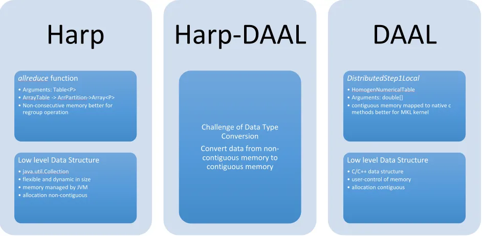
Data Structure of Harp and DAAL

Figure 1. Data structure of Harp and DAAL

Harp defines its own three-level data structure. At the top level is its ArrTbale, which extends the Table class of Java. At the middle level is the ArrPartition, which owns an identifier and an Array. At the low level is the Array that derives from the primitive Array class of Java. Therefore, an ArrTable of Harp could contains a substantial number of ArrPartition, and the data resides on non-consecutive memory space.

DAAL also has a variety of data structures. In general, it has data source, data dictionary, NumericTable, matrix, and so forth. E.g., NumericTable is a major data structure used in DAAL's algorithms. NumericTable has many sub-classes such as HomogenNumericTable, AOSNumericTable, SOANumericTable. In HomogenNumericTable, the data is stored in consecutive chunks of memory space, while the AOSNumericTable has its data stored in non-contiguous memory space. If the users use the Java APIs of these data structures, they could also decide whether the data's memory space is allocated on the Java side or on the C++ side. There are pros and cons for both of the two sides, and we will investigate them in the following sections.

Because of the different data structures, the interface needs to address the data conversion problem, and consequently, will cause additional time overhead. Unless we modify the data structures of Harp and DAAL, we can only use some multithreading copy to reduce the conversion time overhead. The JNI interface used in DAAL's Java APIs will also give us some challenges that will be discussed in the following sections.

Two Case Studies and Preliminary Results

We select two algorithms, K-means and Stochastic Gradient Descent (SGD), to test our interface implementation. K-means represents the category of computation-intensive problems while SGD represents the category of memory-intensive applications.

For each of them, we will compare the performance of the Harp-DAAL interfaced hybrid codes with that of the original pure Java codes.

Harp

allreduce function

• Arguments: Table<P>

• ArrayTable -> ArrPartition->Array<P> • Non-consecutive memory better for

regroup operation

Low level Data Structure

• java.util.Collection • flexible and dynamic in size • memory managed by JVM • allocation non-contiguous

Harp-DAAL

Challenge of Data Type Conversion Convert data from

non-contiguous memory to contiguous memory

DAAL

DistributedStep1Local

• HomogenNumericalTable • Arguments: double[]

• contiguous memory mapped to native c methods better for MKL kernel

Low level Data Structure

Harp-DAAL-Kmeans

The interface between Harp's K-means and DAAL's K-means is quite straightforward.

//--- Harp codes to get pointPartitions ---//

//--- start convert data from Harp to DAAL

---HarpDaalParallelConvert converter = new HarpDaalParallelConvert(pointPartitions, pointData, pointPartition s.size(), pointsPerFile, vectorSize);

converter.HarpToDaal();

HarpDaalParallelConvert converter_cen_to_daal = new HarpDaalParallelConvert(cenTable, daalCenData, numCenP artitions, 0, vectorSize);

converter_cen_to_daal.HarpCenToDaal();

//--- End of converting data from Harp to DAAL ---//

//create the DAAL's data structure

HomogenNumericTable ntData = new HomogenNumericTable(daalContext, pointData, vectorSize, totalVectors); HomogenNumericTable ntCen = new HomogenNumericTable(daalContext, daalCenData, vectorSize, numCentroids); // compute K-means by DAAL

DistributedStep1Local kmeansLocal = new DistributedStep1Local(daalContext, Double.class, Method.defaultDen se, numCentroids);

kmeansLocal.input.set(InputId.data, ntData);

kmeansLocal.input.set(InputId.inputCentroids, ntCen); PartialResult pres = kmeansLocal.compute();

HarpDaalParallelConvert is a defined class that uses Java multithreading to copy data from Harp's pointPartition to DAAL's pointData

In the test, we compiled the codes with the DAAL-2017 released version on Github The test of K-means was done by two mappers on a single node of Juliet. The test of MF-SGD was done by four mappers on two nodes of Juliet.

• Harp-Kmeans

Origianl implementation of Bingjing, the local computatoin kernel of K-means is written in Java multithreading

• Harp-DAAL-Kmeans

Hybrid implementation of Harp with DAAL-2017. The local computation is offloaded to DAAL while the communication layer is handled by Harp. There is a group of Java classes dedicated to the data type conversion between Harp and DAAL

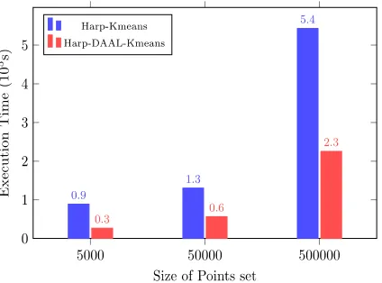
The K-means tests used data points where each point is a vector with a length of 10. Each test had 10 iterations of computing K-means, and each test was repeated by 5 times. Thus, the averaged results could remove the influence from the fluctuation of Hadoop JVM's performance. In order to investigate the benefits of DAAL to Harp-Kmeans, we divided the tests into two groups.

• Group 1: The tests fix the number of data points to 500000 while varying the number of centroids by 1000, 10000, 100000, respectively.

• Group 2: The tests fix the number of centroids to 100000 while varying the number of data points by 5000, 50000, 500000, respectively.

Figure 2. Test Results of Group 1 Figure 3. Test Results of Group 2

In Figure 2., we found that the execution time of both Harp-Kmeans and Harp-DAAL-Kmeans increase rapidly when we augment the number of centroids. The benefits of DAAL is obvious because it saves by 2x to 4x the execution time in average. In Figure 3., Harp-DAAL-Kmeans still saves up to 3 times of the execution time compared to Harp-Kmeans.

Harp-DAAL-SGD

Matrix Factorization based on Stochastic Gradient Descent

Matrix Factorization based on Stochastic Gradient Descent (SGD-MF for short) is an algorithm widely used in recommender systems. MF-SGD is one of the implemented algorithm within Harp, however, DAAL current does not have a MF-SGD kernel. We first implement a MF-SGD kernel inside DAAL's framework and then interface it with that of Harp. MF-SGD aims to factorize a sparse matrix into two dense matrices named mode W and model H as follows.

𝑉 = 𝑊𝐻

Matrix 𝑉 includes both training data and test data, a machine learning inspired kernel with use the training data to approximate the model matrices 𝑊 and 𝐻. A standard SGD procedure will update the model 𝑊 and 𝐻 when it trains each training data, i.e., an entry in matrix 𝑉 in the following formula.

𝐸𝑖𝑗 = 𝑉𝑖𝑗− ∑ 𝑊𝑖𝑘 𝑟

𝑘=0

𝐻𝑘𝑗

𝑊_𝑖∗𝑡 _{= 𝑊}

𝑖∗𝑡−1− 𝜂(𝐸𝑖𝑗𝑡−1⋅ 𝐻∗𝑗𝑡−1− 𝜆 ⋅ 𝑊𝑖∗𝑡−1)

𝐻_∗𝑗𝑡 = 𝐻_∗𝑗𝑡−1− 𝜂(𝐸_𝑖𝑗𝑡−1⋅ 𝑊_𝑖∗𝑡−1− 𝜆 ⋅ 𝐻_∗𝑗𝑡−1)

Tests on Harp-SGD and Harp-DAAL-SGD

Archive of DAAL-MF-SGD on IU's Github

Online Documentation of DAAL-MF-SGD

In the test, we refer the original pure-Java implementation as Harp-SGD while the hybrid one with DAAL's kernel as Harp-DAAL-SGD. We use two nodes from Juliet cluster located at Indiana

University Bloomington in our tests.

Each node has the following CPU information:

Architecture: x86_64 CPU op-mode(s): 32-bit,

64-bit Byte Order: Little Endian CPU(s): 48

On-line CPU(s) list: 0-47 Thread(s) per core: 2 Core(s) per socket: 12

The memory configuration of Harp on each node is shown as follows:

Yarn allocates: 128 GBs Each Mapper allocates: 100 GBs

In the test, we use two datasets.

1.MovieLens 2.Yahoomusic

Total Iteration times: 5 LearningRate: 0.005 Lambda: 0.003 Threads: 40

Total Mapper 2, Each node has 1 mapper

Figure 4. Test on MovieLens with 128 dimensional Feature Vector

Figure 5. Test on Yahoomusic with 128 dimensional Feature Vector

In Figure 4 and 5, we find that, by integrating DAAL's kernel into Harp, the Harp-DAAL-SGD does have less execution time than the original Harp-SGD. However, the performance speedup is only around 6% for Yahoomusic and 16.5% for MovieLens. As we know, Yahoomusic has a larger data size than MovieLens, which indicates that it should have more computation workload. However, the speedup brought by DAAL's computation kernel is less effective on large dataset, which requires a further investigation.

By decomposing the execution time into different stages within Harp-DAAL-SGD, we have the following pie chart:

In Figure 6, we have seen two additional overhead beside computation and data communication between distributed nodes (refers to model rotation).

1.Interfacing Overhead

2.JNI Overhead

They all together take up to 25% of the whole execution time. These overheads do not exist at the pure-Java implementation of Harp-SGD, they are, actually the side-effect of interfacing two languages and two libraries.

Interface Overhead Between DAAL and Harp

DAAL and Harp have their own different data abstracts. DAAL is likely to use contiguous allocated memory either at native side, or at the heap of Java side. In contrast, Harp uses a Table structure, where each of its element is allocated on Java Heap individually. The collective communication functions provided by Harp only supports its own Table structure, therefore, when we need to transfer data, like the updated model 𝑊 and 𝐻 to other nodes, we have to decompose the contiguous table from DAAL into Harp's Table structure. In our Harp-DAAL-SGD implementation, we use Java multi-threading to copy data between the two data containers, and the overhead could be controlled in large data cases.

JNI overhead in data transfer

Another interface overhead is the data transfer between two languages. The model data 𝑊 and 𝐻

are initially created at the heap space of Java, and DAAL's native kernel could not access them directly. In DAAL's Java interface, we have two solutions.

1.Explicitly allocating data at the native code side in Java programming codes. The data is actually allocated at the DirectBuffer of Java, and the memory address of this buffer could be passed to the native kernel of DAAL by JNI interface.

2.Keeping the data at the Java heap side. Each time the native kernel needs to access the data, it will callback to the Java side and temporarily create a DirectBuffer for the required data at the native code side.

Since the MF-SGD kernel will usually update the same model data by a multiple times, we find the first choice has less time overhead than the second one. Therefore, we pass the model data 𝑊 and 𝐻

from Heap side to the DirectBuffer before the computation kernels start. After the computation finishes, we retrieve the updated model data to the Java heap side for rotation. This two-side data transfer contributes a roughly 20% of the total execution time. Java does not have a pointer type as that of C/C++, thus, we could not execute the data transfer between DirectBuffer and Heap segmentation by segmentation in parallel. With the data size increases, the JNI overhead increases accordingly.

Future Work on Harp-DAAL interface

• Re-implement the communication function of Harp, making it compatible to DirectBuffer memory beside the heap memory

• Currently DAAL only has homogeneous table that supports buffer implementation. If the SOANumericTable can also have such buffer implementation support, we may eliminate the data copy from contiguous memory to separated memory space.

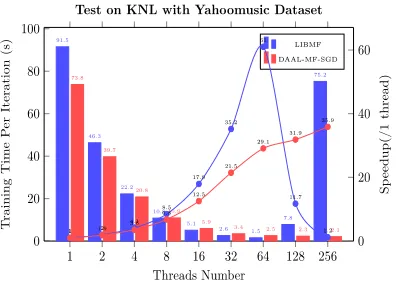
Performance Evaluation of DAAL-SGD-MF and Libmf

Figures 7 and 8 show the comparison of DAAL-SGD-MF and LIBMF. The execution time per iteration shows that LIBMF works faster than DAAL-SGD-MF, however, LIBMF has a worse convergence than DAAL.

We also observe that LIBMF quickly drops out of performance when it runs more than 64 threads, which is the number of physic cores (threads) of our KNL. These differences and phenomena come from the fact that, although both of LIBMF and DAAL follow the same standard SGD algorithm for matrix factorization, they adopt different computation model (synchronization pattern) and multi-threading programming paradigm.

Figure 7.Time per iteration and Threads scalability

Figure 8. Convergence by Timeline

Model Rotation vs. Asynchronous communication

Thread based Scheduling vs. Task based Scheduling

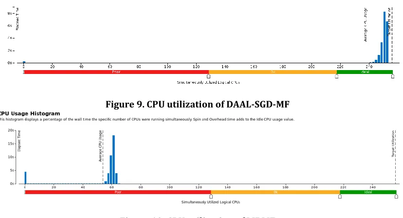
LIBMF uses a raw pthread based multi-threading programming, the developers write their own threads scheduler that follows the model rotation strategy and a dynamic threads scheduling. DAAL-SGD-MF chooses the Task based scheduling, which is accomplished by Intel's TBB library. Though both of them has a dynamic thread scheduling policy, there are some fundamental differences between thread based scheduling and tasks based scheduling. According to an explanation provided by Intel.

The threads you create with a threading package are logical threads, which map onto the physical threads of the hardware. For computations that do not wait on external devices, highest efficiency usually occurs when there is exactly one running logical thread per physical thread. Otherwise, there can be inefficiencies from the mismatch.

This explains the drop down of LIBMF when it uses more than the number of physic threads. DAAL-SGD-MF, thanks to the task-based scheduling by TBB, could take advantage of hyper threading and achieve a higher CPU/Threads utilization than that of LIBMF. (See Figure 9)

Figure 9. CPU utilization of DAAL-SGD-MF

Figure 10. CPU utilization of LIBMF

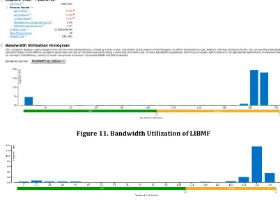
L2 cache hit Rate and Memory Access Latency

Figure 11. Bandwidth Utilization of LIBMF

Figure 12. Bandwidth Utilization of DAAL-SGD-MF

SGD-MF Optimization on KNL

Matrix Factorization is one of the best techniques to solve a collaborative filtering problem in order to build a recommender system. It is a typical big data analysis algorithm, which deal with both large volume of input data (user-item ratings) and large volume of model(user-latent and item-latent matrix).

Libmf1 _{is the state-of-art implementation on multi-threading and share memory platform using SGD} solver for the matrix factorization problem. It builds up by two basic ideas. First, it achieves free-of-conflicts model updates by splitting the input matrix into blocks and using a dynamic scheduler to select blocks without conflicts for the running threads. Second, it re-organizes the processing order of the training points into a more cache friendly way, with a compromise of the randomness required by the algorithm. It’s always a trade-off between efficiency and effectiveness.

In this report, we investigate the performance issue of a sgd-mf trainer on the new KNL

architecture by using libmf. We try to find out the bottleneck of this kind of application and possible solutions. Currently, it has the following sections:

 Performance Evaluation

 Bottleneck Analysis  Optimization

 Optimization By Reorganize Memory Access Order: Tiling  Optimization By Reorganize Memory Layout: Nopermute

 Optimization By Repeat Computation on Training Points: Repeat  Optimization By Decrease Memory Access Latency: NUMA

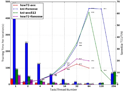
Performance Evaluation of Haswell vs. KNL

Run libmf on the standard yahoomusic dataset, with different thread number under a fixed eta(learning rate), two platform(hsw72, knl), two vectorization optimization(avx512 on/off knl & avx on/off hsw72):

mf-train -l2 1 -k 128 -r 0.0001 -t 10 -s #threadnum -p yahoomusic-test.mm yahoomusic-train.mm

KNL runs with mcdram in flat mode, all datasets are allocated into mcdram.

Figure 13 Performance Evaluation of Libmf

According to Figure13, we have the following observations from this experiment: A). Avx512

a) On knl, avx512 runs about 5x faster than nosse (vectorization off) b) On hsw72, avx runs about 1.6x faster than nosse(vectorization off)

B). Hyper-Threading

b) It goes even worse when vectorization on.

C). Speedup

a) On hsw72, speedup is below the linear, e.g., 21.7 at S32 (thread=32) b) On Knl, speedup is near (super) linear, e.g., 61 at S64.

It seems libmf has better scalability on knl. But the very slow performance of one thread on knl can contribute to this.

D). Performance

a) Each core of Hsw72 is more powerful than the counter part of KNL

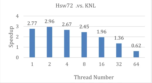
b) But as in Figure 14, the advantage of HSW decreases when more threads are used. Later, we find out that the memory bandwidth on HSW becomes the bottleneck.

Figure 14 Performance Comparison Between HSW and KNL c) KNL finally runs faster

KNL get best performance at 1.5(s/iter) on S64, which is about 1.27x faster than Hsw72’s best preformance of 1.9 on S32.

Bottleneck Analysis

Performance analysis with VTUNE shows that this application has high l2-cache miss rate and low FPU utilization. (see Appendix)

L2 hit rate 0.541

L2 miss bound 1.00

FPU utilization upper bound 10.7%

Bandwidth Utilization MCDRAM flat ~180GB/s

SIMD compute-to-l2 access ratio 24.810

There is a low compute-to-memory load ratio, thus the power of FPU can not be delivered fully.

Then we try different ways to optimize, either to increase the l2 hit rate by reorganize the memory access order or decrease the latency of memory access by utilize the NUMA topology, or increase the computation for each memory load by modifying the algorithm.

2.77 2.96 _{2.67 2.45}

1.96 1.36

0.62

0 1 2 3 4

1 2 4 8 16 32 64

Sp

ee

dup

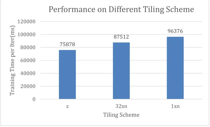
Optimization By Reorganize Memory Access Order: Tiling

Tiling, a better organization of memory access, can be used to make the memory access more cache friendly, thus may ameliorate this kind of memory-bounded problem.

There are different tiling schemes: a) row-based, b)col-based, c)z-filling, (cache oblivious filling). Libmf itself split the input training data matrix into blocks, and do partial random training on the training points by select blocks randomly but select points inside one block with a special order. By default, it uses a row-based order.

First, we test different tiling schemes on libmf with one thread and one block setting, avx512 open.

problem[m=1000990, n=624961,nnz=252800275]

Figure 15 Performance on Different Tiling Scheme

Z filling is about 1.27x faster than non-tiling.

VTune analysis on tiling:

Non-tiling Z-filing

FPU Utilization Upper Bound: 9.0%

GFLOPS Upper Bound: 3.742

Scalar GFLOPS Upper Bound: 0.009

Packed GFLOPS Upper Bound: 3.732

FPU Utilization Upper Bound: 12.3%

GFLOPS Upper Bound: 5.083

Scalar GFLOPS Upper Bound: 0.006

Packed GFLOPS Upper Bound: 5.077

75878

87512 96376

0 20000 40000 60000 80000 100000 120000

z 32xn 1xn

Tr

ain

in

g

Ti

me

pe

r

Ite

r(

ms

)

Tiling Scheme

Back-End Bound: 45.5%

L2 Hit Bound: 0.160

L2 Miss Bound: 1.000

MCDRAM Flat Bandwidth Bound: 0.0%

DRAM Bandwidth Bound: 0.0%

Back-End Bound: 50.4%

L2 Hit Bound: 0.233

L2 Miss Bound: 1.000

MCDRAM Flat Bandwidth Bound: 0.0%

DRAM Bandwidth Bound: 0.0%

CPU Utilization: 0.4%

Average CPU Usage: 0.996 Out of 256 logical CPUs

CPU Utilization: 0.4%

Average CPU Usage: 0.996 Out of 256 logical CPUs

There is minor improvement on L2 hit count, subsequently a small improvement on FPU utilization. But it does not change the L2 Miss Bound anyway. Furthermore, the benefits from z-filing will decrease when the thread number increases, for this application deals with a sparse matrix and there are less chances to reuse the data loaded when the blocks size get smaller.

Optimization By Reorganize Memory Layout: Nopermute

Applying permutation on the rows and columns of the training matrix is a standard pre-process step in Libmf, which can make the load more balance among the threads. However, the randomness from permutation make the cache harder to work efficiently.

Here we try skip the permutation in preproces, and on the contrary, we reorder the rows and columns by their frequency of non-zero items in each block. And following the idea of partial randomness in libmf, we rely on the dynamic scheduler randomly select blocks to make the converge rate not deteriorate much comparison with the totally random training point selection.

Thread=64, Blocks=129, Iternum=10

With Permutation Nopermute(ms) Nopermute(ms)+z-filing

TrainTime/Iter(ms) 1490 1280

Test RMSE 26.1194 26.1604

It can achieve about 10% times faster by nopermute, but not much.

Optimization By Repeat Computation on Training Points: Repeat

Here we do repeat computation on a chunk of training data to increase the data reuse and the computation-to-memload ratio.

Parameters:

chunksize How many points will be retrained as a group/chunk

repeatcnt How many times the chunk data will be retrained

VTune Profiling

S64N0,xtile=3, repeat=3,chunksize=16 S64N0,xtile=3 no repeat

CPU Utilization: 24.8%

Average CPU Usage: 63.546 Out of 256 logical CPUs

CPU Utilization: 21.4%

Average CPU Usage: 54.850 Out of 256 logical CPUs

L2 Hit Bound: 0.088

L2 Miss Bound: 0.640

MCDRAM Flat Bandwidth Bound: 0.0%

DRAM Bandwidth Bound: 0.0%

L2 Hit Bound: 0.148

L2 Miss Bound: 1.000

MCDRAM Flat Bandwidth Bound: 0.0%

DRAM Bandwidth Bound: 0.0%

FPU Utilization Upper Bound: 15.3%

GFLOPS Upper Bound: 405.943

Scalar GFLOPS Upper Bound: 0.450

Packed GFLOPS Upper Bound: 405.493

FPU Utilization Upper Bound: 10.5%

GFLOPS Upper Bound: 239.319

Scalar GFLOPS Upper Bound: 0.206

Packed GFLOPS Upper Bound: 239.113

Top 5 hotspot loops (functions) by FPU usage

Function CPU Time FPU Utilization Upper Bound Loop Characterization

[Loop@0x41eeb2 in mf::(anonymous namespace)::SolverBase::run] 1512.121s 7.7%

[Loop@0x41f1a0 in mf::(anonymous namespace)::SolverBase::run] 1268.951s 25.2%

[Loop@0x41efc5 in mf::(anonymous namespace)::SolverBase::run] 1233.001s 2.2%

mf::(anonymous namespace)::Block::move_next 611.510s 21.9%

[Loop@0x41f1f8 in mf::(anonymous namespace)::SolverBase::run] 607.590s 41.1%

[Others] 120.650s N/A*

Top 5 hotspot loops (functions) by FPU usage

Function CPU Time FPU Utilization Upper Bound Loop Characterization

[Loop@0x41e375 in mf::(anonymous namespace)::SolverBase::run] 1133.191s 1.0%

[Loop@0x41e262 in mf::(anonymous namespace)::SolverBase::run] 495.050s 8.7%

[Loop@0x41e550 in mf::(anonymous namespace)::SolverBase::run] 424.420s 23.9%

[Loop@0x41e5a8 in mf::(anonymous namespace)::SolverBase::run] 196.480s 40.8%

mf::(anonymous namespace)::Block::move_next 88.750s 9.6%

[Others] 114.550s N/A*

From the VTUNE report, the Repeat technique can really increase the FPU utilization and decrease the l2 miss bound in the back-end.

TestRMSE iter avg time(ms) Total(ms) speedup chunksizeXrep eatcnt

24.1733 17 1773 30141 1

9 1961 17649 1.707802142 8x1

6 2460 14760 2.042073171 8x2

5 3088 15440 1.952137306 8x3

This table shows the speedup by “repeat” to converge to the same level in training with different repeatcnt settings.

But another group experiments with different chunksize settings show little differences in terms of performance. It means, we can not benefit more from repeat on a larger chunk of points than repeat on a single point. The problem here is that repeat on a single point actually has little differences with doubling the learning rate parameter. Thus, the repeat technique doesn’t work effectively on such kind of sparse problem.

Optimization By Decrease Memory Access Latency: NUMA

Because this application is memory-bound with high l2-miss rate, we can try to decrease the memory access latency by utilize the topology information of the numa architecture.

Performance Evaluation of Harp-SGD-MF on KNL

Learning parameters

Number of Training Points 252800275 Number of Rows: 1000990

Number of columns: 624961 Number of Dimensions: 100 Lambda: 1

Epsilon: 0.0001

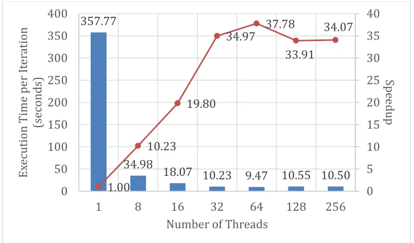
The results are shown in the chart below. There is (super) linear speedup on 1, 8, 16 and 32 threads. However, the speedup couldn’t grow when the number of threads is higher than 32 because the computation time doesn’t change much.

Figure 16 Performance Evaluation of Harp SGD for MF

Appendix

VTUNE Analysis Report Libmf Parameters

Thread number: 64 K: 128 Lambda: 1 Eta: 0.0001 AVX512: on MCDRAM: on VTune--General info

357.77

34.98

18.07 10.23 9.47 10.55 10.50

1.00

10.23

19.80

34.97

37.78

33.91

34.07

0

5

10

15

20

25

30

35

40

0

50

100

150

200

250

300

350

400

1

8

16

32

64

128

256

Sp

ee

dup

Ex

ecuti

on

T

ime p

er I

ter

at

ion

(second

s)