Time-delayed autosynchronous swarm control

Time-delayed auto-synchronous swarm control

James D. Biggs, Derek J. Bennet, and S. Kokou Dadzie [email protected], Advanced Space Concepts Laboratory,

Department of Mechanical & Aerospace Engineering, University of Strathclyde, Glasgow.

(Dated: January 5, 2012)

Abstract

In this paper a general Morse potential model of self-propelling particles is considered in the

presence of a time-delayed term and a spring potential. It is shown that the emergent swarm

behavior is dependent on the delay term and weights of the time-delayed function which can be set

to induce a stationary swarm, a rotating swarm with uniform translation and a rotating swarm with

a stationary center-of-mass. An analysis of the mean field equations shows that without a spring

potential the motion of the center-of-mass is determined explicitly by a multi-valued function. For

a non-zero spring potential the swarm converges to a vortex formation about a stationary

center-of-mass, except at discrete bifurcation points where the center-of-mass will periodically trace an

ellipse. The analytical results defining the behavior of the center-of-mass are shown to correspond

I. INTRODUCTION

In nature swarms of social entities such as insects, birds and fish, self-organize through local communications as opposed to centralized behavioral control. Mathematical investi-gations into the emergent spatio-temporal patterns of such swarms have been used to gain an understanding of the mechanism that drives this natural phenomena1–7_{. In turn this} re-search has led to a number of efficient algorithms designed to control swarms of autonomous systems8–13_.

Many different mathematical approaches have been used to describe de-centralized swarm behavior. A common approach to modeling coherent swarms is in the use of Artificial Po-tential Functions (APFs)12–19_{. APFs have gained popularity in algorithms for de-centralized} swarm control of autonomous systems as they are simple to implement, their emergent be-havior is often verifiable analytically, see for example,21 _{and they can be used for obstacle} avoidance22_.

This paper focusses on approaches that have been used to model rotation in swarms of self-propelled particles which are either translating or with a stationary center-of-mass23–25_. These models23–25 _{all use APFs combined with additional terms to induce rotating swarms.} In McInnes23 _{a Morse APF was combined with a velocity alignment function requiring} in-formation on the relative velocity of each particle to induce vortex in-formations. In Ebeling. et al.24 _{it was shown that a translating swarm induced by a harmonic attractive APF} tran-sitioned to a rotational motion in the presence of noise (with a large enough intensity) and in Schwartz and Forgotson25 _{a purely attractive APF in the presence of noise and the} addi-tion of a communicaaddi-tion time-delay was investigated. This showed that the delay induced transition from translational to rotational motion was associated with a super-critical hopf bifurcation as the value of a coupling parameter was increased. The models used by24,25 have a computational advantage over the model in23 _{as the swarm control algorithms do} not require information on the relative velocity. However, the model in23 _{is deterministic} and the mean field equations can be investigated without imposing assumptions such as the equivalence of deterministic averaging and statistical averaging or simply ignoring the stochastic perturbations.

parameter is introduced into the equations, but in this case it is a delay in a velocity term rather than a delay in the relative position of each particle. The delay in25 _{is introduced to} account for communication time delays. However, the delay term here is considered purely as a feedback mechanism26,27 _{requiring the ability to sense current state and store information} on historical state. An investigation of the effect of a time-delay directly on an APF without the presence of noise is undertaken. It is shown that noise is not required to induce rotational motion with a stationary center-of-mass and can be a purely delay dependent phenomena. In comparison to previous deterministic algorithms to induce vortex formations in self-propelled particles this method does not require relative velocity information so is computationally more efficient. Furthermore, the completely deterministic mean field equations are shown to be linear delay differential equations that allow a complete stability analysis to be undertaken without the need for sophisticated numerical tools.

We consider a two-dimensional (2-D) model of a swarm that consists of homogeneous, self-propelled agents (1≤i≤N) that are interacting through the following APF, U(xi):

U(xi) =

X

j,j6=i



 Crexp

−|xij|

Lr −C_aexp

−|xij|

La



 +β

m_i

2 |xi(t)| 2

(1)

where,xi is the position vector of agentiwith corresponding massmi and xij is the relative

position vector of agentsi andj,Ca,Cr andLa,Lr represent the amplitude and range of the

attractive and repulsive potential respectively. Two cases of the APF are considered when

β = 0 and β = 1. The Morse potential (Equ. (1) withβ = 0) is used to provide long-range attraction and weak short-range repulsion (collision-free motion) for the swarm of agents? _. The spring potential (mi

2 |xi(t)|2) is used to bound the motion of the swarm about the origin.

The swarm behavior is induced by the following equations of motion

˙

xi =vi (2)

where vi defines the mechanism of self-propulsion and

miv˙i =−∇iU(xi) +ui(t), (3)

where,

with a and b are arbitrary constants and τ a delay term. The dissipation term (4) is of the form of a time-delayed feedback control or time-delayed auto synchronization (T-DAS) a method originally posed by Pyragas26_{. The following section considers the case when}

β = 0 (no spring potential) and investigates the interaction between T-DAS and the Morse potential function.

II. SIMULATION AND ANALYSIS FOR β = 0

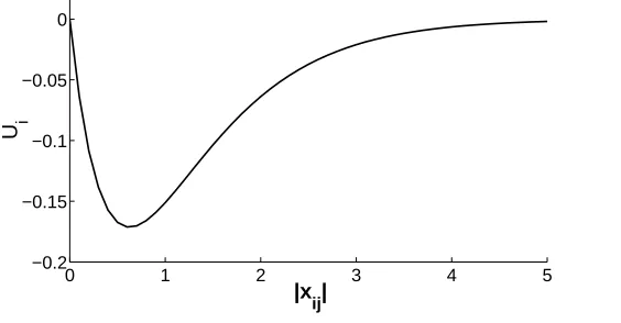
For this study the parameters of the potential function are taken to beβ = 0, Ca= 1, La =

0.8, Cr = 1, Lr = 0.5 which yields the potential function illustrated in Figure 1 Numerical

0 1 2 3 4 5

−0.2 −0.15 −0.1 −0.05 0

|x

ij|

U i

(i)

FIG. 1: The Morse potential as a function of agent separation

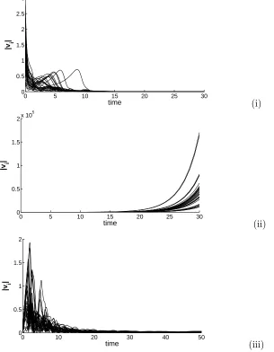
simulations were undertaken for agents in the x-y plane. An example is given in Fig. 2 where the velocity of each agent is illustrated. In Figure 2 (i) b > a whereby the feedback control magnitude and direction is dominated by its current velocity. As the feedback control acts in the opposite direction to the current velocity it will act as a dissipative force and the speed of each agent will converges to zero i.e. the center-of-mass stops. In Figure 2 (ii) a > b

0 5 10 15 20 25 30 0 0.5 1 1.5 2 2.5 3 time |v i | (i)

0 5 10 15 20 25 30

0 0.5 1 1.5

2x 10

5

time

|v i

|

(ii)

0 10 20 30 40 50

0 0.5 1 1.5 2 time |v i | (iii)

FIG. 2: The magnitude of the velocity history for 30 agents in the swarm given by numerical

simulation with random initial conditions (i) b > a all velocities converge to zero (asymptotically

stable) (ii)a > bthe velocities diverge rapidly (unstable) (iii)a=bthe velocities are non-zero but

bounded (marginally-stable)

field equations. The mean field equations are derived by defining the position Rc, velocity

˙

Rc and acceleration ¨Rc of the center-of-mass of the swarm by Eq. (5)

Rc =

X

i mixi

X

i mi

, R˙c =

X

i mivi

X

i mi

, R¨c =

X

i miv˙i

X

i mi

then summing over all agents in Eq. (3), with delay term (4) included, yields X

i

m_iv˙i(t) =−b

X

i

m_ivi(t) +a

X

i

m_ivi(t−τ), (6)

where, P

i∇iU(xij) = 0 due to internal symmetry in the swarm. The center-of-mass of

the swarm can, thus, be expressed combining equations (5) and (6) to yield the mean field equations:

¨

Rc(t) =aR˙c(t−τ)−bR˙c(t), (7)

which after using the change of variable,

x(t) = ˙Rc(t) and ˙x(t) = ¨Rc(t), (8)

is rewritten as

˙

x(t) =−bx(t) +ax(t−τ). (9)

The stability analysis of this equation will then determine the behavior of the center-of-mass of the swarm. Assuming equation (9) to have a wave function as a solution of the form,

x(t) = eλkt with _λ

k a complex number, then the characteristic equation associated with

equation (9) is:

λk =−b+ae−λkτ (10)

The solution to the transcendental equation (10) can be given analytically in terms of a Lam-bert function, as is well known for a one-dimensional linear time-delay differential equation27_. By definition, the Lambert function W(z), is a multi-valued function given implicitly by equation

z =W(z)eW(z), (11)

with z any complex number.

So, equation (10) is first rewritten as

τ λkeλkτ =τ −beλkτ +a

, (12)

then into

(bτ +λkτ)eλkτebτ =aτ ebτ, (13)

or

(bτ +λ_kτ)eλkτ+bτ

From the definition of the Lambert function in equation (11), the solution to equation (14), is

bτ +λkτ =W(aτ ebτ). (15)

or

λk =

−bτ +W(aτ ebτ₎

τ . (16)

Therefore, knowing properties of the Lambert function one can analyze the solution of equa-tion (16) of the characteristic equaequa-tion (10) and extract stability criteria which is primarily defined as Re[λk] < 0 for all λk. As a multi-valued function, the branches or the set of

Lambert functions are denoted Wk(z) with k ∈ Z. For a given triplet, (b, a, τ), the set of

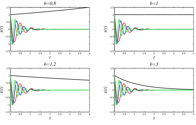
solutions in equation (16) admits a clear leading eigenvalue, the rightmost eigenvalue. The value of this rightmost eigenvalue, that is given byλ₀, by conjecture determines the stability i.e. Re[λ0]<0 implies the center-of mass will converge. Fig. 3 illustrates a surface (a= 1) with the vertical axes corresponding to the real part of the right-most eigenvalue of the sys-tem, and the horizontal axis the parameterb and the delayτ. This illustrates the stable and unstable regions of the swarm, that is, when the center-of-mass stops and when it diverges rapidly. The eigen-modes for a subset of these values are also illustrated in Figure 4. This indicates that, in all cases, all of the eigen-modes converge to zero except in the case of the right-most eigen-mode which is the controlling mode. However, the right-most eigen-mode is dependent on the values of the parameters a and b as is illustrated. The equation of the velocity of the centre-of-mass (recallx(t) = ˙Rc(t)) can also be explicitly defined as a solution

of the Delay Differential Equation (DDE) equation (9) by,

x(t) = +∞ X

k=−∞

C_keλkt_.

(17)

where λ_k is defined by Equ. (16) and the coefficients C_k are dependent on the initial conditions.

III. SIMULATION AND ANALYSIS FOR _{β= 1}

-0 0.5 1 1.5 2 −5 −4 −3 −2 −1 0 1 2 3 4 5 −4 −3 −2 −1 0 1 2 3 4 5 6 b τ Re[ λ 0 ]

FIG. 3: (Color online) Real part of the right-most eigenvalue is represented by the multi-colored

surface (grayscale surface in print) with varyingbandτ intersecting the plane defined byRe[λ0] = 0 represented by the single colored surface (black surface in print)

0 0.5 1 1.5 2 2.5 3 3.5 4

−1.5 −1 −0.5 0 0.5 1 1.5 b=0.8 t x(t)

0 0.5 1 1.5 2 2.5 3 3.5 4

−1.5 −1 −0.5 0 0.5 1 1.5 b=1 t x(t)

0 0.5 1 1.5 2 2.5 3 3.5 4

−1.5 −1 −0.5 0 0.5 1 1.5 b=1.2 t x(t)

0 0.5 1 1.5 2 2.5 3 3.5 4

−1.5 −1 −0.5 0 0.5 1 1.5 b=3 t x(t)

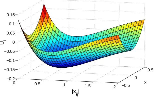
bounded velocity) or unstable (exponentially diverging velocity). In this section we investi-gate the transition of these swarm topologies to rotating swarms with a stationary center-of-mass due to the addition of a spring potential. It is shown that introducing a spring potential alongside the Morse potential, and used in combination with T-DAS, induces dy-namic vortex formations about the origin. The spring potential function is purely attractive and grows linearly with the separation between each particle and the origin. Explicitly the APF (1) is used with β = 1, C_a = 1, L_a = 0.8, C_r = 1, L_r = 0.5 which yields the potential function surface in Figure 5. Note that for b > athe velocities will always converge to zero

0 _{0.5 1}

1.5 ₂ −0.5

0 0.5

−0.2 −0.15 −0.1 −0.05 0 0.05 0.1 0.15

x

|x

ij|

U i

FIG. 5: (Color online) The potential surface as a function of agent separation and the distance x

from the origin

0 10 20 30 40 50 0 1 2 3 4 time |v i | (i)

0 20 40 60 80 100

0 0.5 1 1.5 2 time |v i | (ii)

FIG. 6: The velocity magnitude history for 30 agents in the swarm (i) a=b= 1 all velocities are

small and bounded (ii) a= 1.1, b= 1 velocities are bounded but their magnitudes become larger

all agents in Equ. (3) with β = 1 yields: X

i

miv˙i(t) =−

X

i

mivi(t) +

X

i

mivi(t−τ)−

X

i

mixi (18)

where P

i

xi is the additional component to the previous case (6) corresponding to the

ad-dition of the spring potential andP

i∇iU(xij) = 0 due to internal symmetry in the swarm.

The center-of-mass of the swarm can thus be expressed as: ¨

Rc(t) =−R˙c(t) + ˙Rc(t−τ)−Rc(t) (19)

definingX= [Rc(t),R˙c(t)]T, this can be expressed as a linear time delay system of the form:

˙

X(t) = 



0 1

−1 −1 

X(t) + 

 0 0 0 1



X(t−τ) (20)

as the system, shown in equation (20), is of the form ˙X(t) = A0X(t) +A1X(t−τ) where

X(t) ∈ R2 _{can be expressed as X(t) =}

∞ P

−∞

Ckeλkt and A0, A1 ∈ R2×2 are real matrices and 0< τ that the substitution of a sample solution of the formeλkt_v where_v ∈_C2×1\{0}leads

to the characteristic equation:

det ∆(λ_k) = 0 (21)

where,

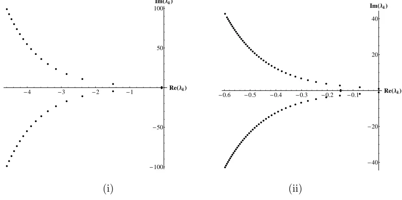
∆(λk) =λI −A0−A1e−λkτ. (22) The particular case when τ = 1 and τ = 2π is illustrated in Figure 7 where the maximum real part of all the eigenvalues isRe(λ₀) = −0.0638512 and Re(λ₀) = 0 respectively. Figure

-4 -3 -2 -1

ReHΛ_kL

-100

-50

50 100

ImHΛkL

-0.6 -0.5 -0.4 -0.3 -0.2 -0.1

ReHΛkL

-40

-20

20 40 ImHΛkL

(i) (ii)

FIG. 7: Characteristic roots of equation (21) for (i) τ = 1 the right most eigenvalue has negative

real part (ii) τ = 2π the two right most eigenvalues lie on the imaginary axis

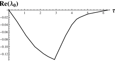
7 illustrates that the center-of-mass will always stop, independently of the number of agents in the swarm, for τ = 1. Figure 8 shows a plot of just the right-most eigenvalue against

1 2 3 4 5 6 Τ

-0.12

-0.10

-0.08

-0.06

-0.04

-0.02

ReHΛ_0L

FIG. 8: The rightmost characteristic roots of the system (20) as a function of the delay term τ

lie on the imaginary axis. In this case ast → ∞all modes converge to zero except the right-most and therefore the solution in the limit is a periodic motion. This periodic solution exists for τ = 2nπ where n∈Z _{and is easily shown to be:}

Rc(t) = ˙Rc(0) sint+Rc(0) cost. (23)

This periodic motion can be considered stable in that all transient motion independently of initial conditions will converge to it (except for the trivial case ˙Rc(0) =Rc = 0). In this case

each agent winds round the origin as illustrated in Figure 10 (ii) with the periodic motion of the center-of-mass tracing an ellipse. If a numerical continuation of the delay parameter is extended beyond τ = 2π it is seen that the real part of the right-most eigenvalue is always negative except at the discrete bifurcation points τ = 2nπ. Note that the bifurcations involve two stable delay-dependent steady states: an equilibrium point and a periodic orbit. However, the eigenvalues never cross the imaginary axis of the complex plane for any value of the delay parameter so it is different from the classical hopf bifurcation reported in Schwartz and Forgotson25_.

IV. CONCLUSION

−0.8 −0.4 0 0.4 0.8 −0.8

−0.4 0 0.4 0.8

x

y

−0.8 −0.4 0 0.4 0.8

−0.8 −0.4 0 0.4 0.8

x

y

(i) (ii)

−0.8 −0.4 0 0.4 0.8

−0.8 −0.4 0 0.4 0.8

x

y

−0.8 −0.4 0 0.4 0.8

−0.8 −0.4 0 0.4 0.8

x

y

(iii) (iv)

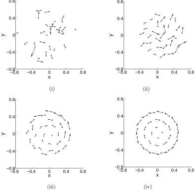
FIG. 9: Swarm of 30 agents forming a vortex independently of initial conditions (i) random initial

conditions (ii) t=10 (iii) t=20 (iv) t=40

−2 −1 0 1 2 −2

−1.5 −1 −0.5 0 0.5 1 1.5 2

y

−0.8 −0.4 0 0.4 0.8

−0.8 −0.4 0 0.4 0.8

x

y

(i) (ii)

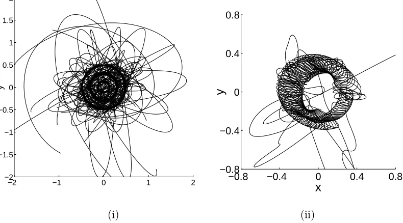
FIG. 10: Trajectories of 30 agents with random initial conditions converging to a steady state (i)

τ = 1 the center-of-mass stops and the swarm forms a vortex formation (ii)τ = 2π the

center-of-mass oscillates about the origin and each agent winds around the origin

requirement as the active interaction only requires that each agent is capable of sensing their relative position within their environment without the need for any relative velocity information. This shows that it is possible to induce rotational motion with a stationary center-of-mass without using noise or information on the relative velocity. Therefore, these results may prove useful in controlling swarms of autonomous vehicles which posses only low-computational power on-board. The model could also provide a deterministic insight into swarm alignment of biological systems such as vortex formation in schools of fish using a feedback mechanism that is a function of memory.

1 _{E. Bonabeau, M. Dorigo, and G. Theraulaz. Swarm intelligence: from natural to artificial}

systems. Oxford, New York, USA, 1999.

2 _{L. Edelstein-Keshet, J. Watmough, and D. Grunbaum. Do travelling band solutions describe}

cohesive swarms? an investigation for migratory locusts. Journal of mathematical biology,

36:515–549, 1998.

21(4):25–34, 1987.

4 _{F. Heppner and U. Grenander. A stochastic non-linear model for coordinated bird flocks. In}

S. Krasner, editor, The Ubiquity of Chaos, pages 233–238. Washington AAAS Publications,

1990.

5 _{H.J. Jenson.Self-Organized Criticality: Emergent Complex Behaviour in Physical and Biological}

Systems. Cambridge University Press, 1998.

6 _{A. Dussutour, V. Fourcassi, D. Helbing, and J-L. Deneubourg. Optimal traffic organization in}

ants under crowded conditions. Nature, 428:70–33, 2004.

7 _{R.S. Miller and W. Stephen. Spatial relationships in flocks of sandhill cranes.Ecology, 47(2):323–}

327, 1966.

8 _{R. Gross, M. Bonani, F. Mondada, and M. Dorigo. Autonomous self-assembly in a swarm-bot.}

IEEE Transactions on Robotics, 22(6):1115–1130, 2006.

9 _{W.J. Crowther. Flocking of autonomous unmanned air vehicles. Aeronautical Journal,}

107(1068):99–110, 2003.

10 _{C.R. McInnes. Velocity field path-planning for single and multiple unmanned aerial vehicles.}

The Aeronautical Journal, 107(1073):419–426, 2003.

11 _{S.W. Ekanayake and P.N. Pathirana. Formations of robotic swarm: An artificial force based}

approach. International Journal of Advanced Robotic Systems, 6(1), 2009.

12 _{D.J. Bennet and C.R. McInnes. Distributed control of multi-robot systems using bifurcating}

potential fields. Robotics and Autonomous Systems, 58(3), 2010.

13 _{A. Badawy and C.R. McInnes. On-orbit assembly using superquadric potential fields. Journal}

of Guidance, Control, and Dynamics, 31(1):30–43, 2008.

14 _{J.H. Reif and H. Wang. Social potential fields: A distributed behavioral control for autonomous}

robots. Robots and Autonomous Systems, 27(3):171–194, 1999.

15 _{V. Gazi and K.M. Passino. A class of attraction/repulsion functions for stable swarm}

aggrega-tions. In Proceedings of the 41st IEEE Conference on Decision and Control, volume 3, pages

2842–2847, Las Vegas, Nevada, USA, December 2002.

16 _{D.E. Chang, S.C. Shadden, J.E. Marsden, and R. Olfati-Saber. Collision avoidance for multiple}

agent systems. In Proceedings of 42nd IEEE Conference on Decision and Control, volume 1,

tive gradient climbing in a distributed environment. IEEE Transactions on Automatic Control,

49(8):1292–1302, 2004.

18 _{D.H. Kim, H. Wang, and S. Shin. Decentralized control of autonomous swarm systems using}

artificial potential functions: Analytical design guidelines. Journal of Intelligent and Robotic

Systems, 45(4):369–394, 2006.

19 _{D. Bennet, J. Biggs, C. McInnes, and M. Macdonald. An analysis of dissiptation functions in}

swarming systems. 18th IFAC Symposium on Automatic Control in Aerospace, 2010.

20 _{M.R. D’Orsogna, Y.L. Chuang, A.L. Bertozzi, and S. Chayes. Self-propelled particles with}

soft-core interactions: Patterns, stability and collapse. Physical Review Letters, 96(10):104302,

2006.

21 _{M.H. Mabrouk and C.R. McInnes. Non-linear stability of vortex formation in swarms of}

inter-acting particles. Phys. Rev. E, 78(1):012903, Jul 2008.

22 _{O. Khatib. Real-time obstacle avoidance for manipulators and mobile robots. The International}

Journal of Robotics Research, 5(1):90–98, 1986.

23 _{C.R. McInnes. Vortex formation in swarms of interacting particles. Physical Review E:}

Statis-tical, Non-linear, and Soft Matter Physics, 75(3):032904, 2007.

24 _{Ebeling W. Mikhailov A. Erdmann, U. Noise-induced transition from translational to rotational}

motion of swarms. Phys. Rev E, 71(051904), 2005.

25 _{Schwartz I. B. Forgotson, E. Delay-induced instabilities in self-propelling swarms. Phys. Rev}

E, 77(035203), 2008.

26 _{K. Pyragas. Continuous control of chaos by self-controlling feedback. Phys. Lett. A., 170(6):421–}

428, 1992.

27 _{P. Hovel. Control of complex nonlinear systems with delay. Springer Theses, 2010.}

28 _{E Jarlebring and T Damm. The lambert w function and the spectrum of some multidimensional}

time-dleay systems. Automatica, 43:2124 2128, 2007.

29 _{W. Michiels and S. Niculescu. Stability and stabilization of time-delay systems: An}