Time-delayed autosynchronous swarm control

Time-delayed autosynchronous swarm control

James D. Biggs,*Derek J. Bennet, and S. Kokou Dadzie

Advanced Space Concepts Laboratory, Department of Mechanical and Aerospace Engineering, University of Strathclyde, Glasgow, United Kingdom

(Received 10 June 2011; revised manuscript received 15 September 2011; published 10 January 2012) In this paper a general Morse potential model of self-propelling particles is considered in the presence of a time-delayed term and a spring potential. It is shown that the emergent swarm behavior is dependent on the delay term and weights of the time-delayed function, which can be set to induce a stationary swarm, a rotating swarm with uniform translation, and a rotating swarm with a stationary center of mass. An analysis of the mean field equations shows that without a spring potential the motion of the center of mass is determined explicitly by a multivalued function. For a nonzero spring potential the swarm converges to a vortex formation about a stationary center of mass, except at discrete bifurcation points where the center of mass will periodically trace an ellipse. The analytical results defining the behavior of the center of mass are shown to correspond with the numerical swarm simulations.

DOI:10.1103/PhysRevE.85.016105 PACS number(s): 05.65.+b, 02.30.Ks, 02.30.Yy, 05.45.Xt

I. INTRODUCTION

In nature swarms of social entities, such as insects, birds, and fish, self-organize through local communications as opposed to centralized behavioral control. Mathematical investigations into the emergent spatiotemporal patterns of such swarms have been used to gain an understanding of the mechanism that drives this natural phenomenon [1–7]. In turn this research has led to a number of efficient algorithms designed to control swarms of autonomous systems [8–13].

Many different mathematical approaches have been used to describe decentralized swarm behavior. A common approach to modeling coherent swarms is in the use of artificial potential functions (APFs) [12–19]. APFs have gained popularity in algorithms for de-centralized swarm control of autonomous systems as they are simple to implement, their emergent behavior is often verifiable analytically, see for example [20], and they can be used for obstacle avoidance [21].

This paper focuses on approaches that have been used to model rotation in swarms of self-propelled particles that are either translating or have a stationary center of mass [22–24]. These models [22–24] all use APFs combined with additional terms to induce rotating swarms. In McInnes [22] a Morse APF was combined with a velocity alignment function requiring information on the relative velocity of each particle to induce vortex formations. In Ebelinget al. [23] it was shown that a translating swarm induced by a harmonic attractive APF transitioned to a rotational motion in the presence of noise (with a large enough intensity), and in Schwartz and Forgotson [24] a purely attractive APF in the presence of noise and the addition of a communication time delay was investigated. This showed that the delay-induced transition from translational to rotational motion was associated with a supercritical Hopf bifurcation as the value of a coupling parameter was increased. The models used by [23,24] have a computational advantage over the model in [22] as the swarm control algorithms do not require information on the relative velocity. However, the model in [22] is deterministic, and the mean field equations

*_{[email protected]}

can be investigated without imposing assumptions, such as the equivalence of deterministic averaging and statistical averaging, or simply ignoring the stochastic perturbations.

In this paper a method for inducing rotational motion of a swarm that interacts via APFs and time-delay autosynchro-nization (TDAS) [25] is presented. Similar to [24] a delay parameter is introduced into the equations, but in this case it is a delay in a velocity term rather than a delay in the relative position of each particle. The delay in [24] is introduced to account for communication time delays. However, the delay term here is considered purely as a feedback mechanism [25,26], requiring the ability to sense the current state and store information on the historical state. An investigation of the effect of a time delay directly on an APF without the presence of noise is undertaken. It is shown that noise is not required to induce rotational motion with a stationary center of mass and can be a purely delay dependent phenomena. In comparison to previous deterministic algorithms to induce vortex formations in self-propelled particles this method does not require relative velocity information, so it is computationally more efficient. Furthermore, the completely deterministic mean field equa-tions are shown to be linear delay differential equaequa-tions that allow a complete stability analysis to be undertaken without the need for sophisticated numerical tools.

We consider a two-dimensional (2D) model of a swarm that consists of homogeneous, self-propelled agents (1iN) that are interacting through the following APF,U(xi):

U(xi)=

j,j₌i

⎡ ⎢ ⎣Crexp

−|xij|

Lr −Caexp −|xij|

La

⎤ ⎥ ⎦+βmi

2 |xi(t)| 2_,

(1)

motion) for the swarm of agents [27]. The spring potential [mi

2|xi(t)|

2_{] is used to bound the motion of the swarm about}

the origin. The swarm behavior is induced by the following equations of motion:

˙

xi =vi, (2)

wherevi defines the mechanism of self-propulsion, and

miv˙i = −∇iU(xi)+ui(t), (3)

where

ui(t)=amivi(t−τ)−bmivi(t), (4)

wherea andbare arbitrary constants andτ is a delay term. The dissipation term (4) is of the form of a time-delayed feedback control or TDAS, a method originally posed by Pyragas [25]. The following section considers the case when

β=0 (no spring potential) and investigates the interaction between TDAS and the Morse potential function.

II. SIMULATION AND ANALYSIS FORβ=0 For this study the parameters of the potential function are taken to be β =0,Ca =1,La =0.8,Cr =1, and Lr = 0.5, which yield the potential function illustrated in Fig. 1. Numerical simulations were undertaken for agents in thex-y

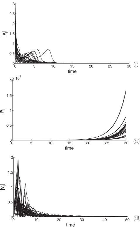
plane. An example is given in Fig.2, where the velocity of each agent is illustrated. In Fig. 2 (i) b > a, whereby the feedback control magnitude and direction are dominated by its current velocity. As the feedback control acts in the opposite direction to the current velocity, it will act as a dissipative force, and the speed of each agent will converge to zero, i.e., the center of mass stops. In Fig.2(ii)a > b, and the feedback control mechanism is dominated by the delayed velocity. As this component of the feedback acts in the same direction as the agent’s motion, the magnitude of velocity will continuously increase. In this case the center of mass diverges exponentially. At the bifurcation pointa=b the velocity of each agent is nonzero yet bounded, as illustrated in Fig. 2 (iii), with the swarm converging to a uniform rotating and translating motion. This qualitative behavior can be characterized by the stability of the center of mass. Furthermore, the behavior of the center of mass can be verified analytically by analyzing the swarm’s mean field equations. The mean field equations are derived by

0 1 2 3 4 5

−0.2 −0.15 −0.1 −0.05 0

|x

ij|

U i

FIG. 1. The Morse potential as a function of agent separation.

0 5 10 15 20 25 30

0 0.5 1 1.5 2 2.5 3

time |v i

|

(i)

0 5 10 15 20 25 30

0 0.5 1 1.5

2x 10

5

time |v i

|

(ii)

0 10 20 30 40 50

0 0.5 1 1.5 2

time |v i

|

(iii)

FIG. 2. The magnitude of the velocity history for 30 agents in the swarm given by numerical simulation with random initial conditions: (i) b > a, all velocities converge to zero (asymptotically stable), (ii)a > b, the velocities diverge rapidly (unstable), and (iii)a=b, the velocities are nonzero but bounded (marginally stable).

defining the positionRc, velocity ˙Rc, and acceleration ¨Rcof the center of mass of the swarm as

Rc= i

mixi

imi

, R˙c= i

mivi

imi

, R¨c= i

miv˙i

imi

. (5)

Then summing over all agents in Eq. (3), with delay term (4) included, yields

i

miv˙i(t)= −b

i

mivi(t)+a

i

mivi(t−τ), (6)

where i∇iU(xij)=0 due to internal symmetry in the swarm. The center of mass of the swarm can thus be expressed by combining Eqs. (5) and (6) to yield the mean field equation:

¨

Rc(t)=aR˙c(t−τ)−bR˙c(t), (7)

which, after using the change of variable,

0 0.5 1 1.5 2

−5 −4 −3 −2 −1 0 1 2 3 4 5 −4

−3 −2 −1 0 1 2 3 4 5 6

b

τ

Re[

λ0

]

FIG. 3. (Color online) Real part of the rightmost eigenvalue is represented by the multicolored surface (grayscale surface) with varying b and τ intersecting the plane defined by Re[λ0]=0, represented by the single colored surface (black surface).

is rewritten as

˙

x(t)= −bx(t)+ax(t−τ). (9)

The stability analysis of this equation will then determine the behavior of the center of mass of the swarm. Assuming Eq. (9) to have a wave function as a solution of the formx(t)=

eλkt _withλ

k being a complex number, then the characteristic

equation associated with equation (9) is

λk= −b+ae−λkτ. (10)

The solution to the transcendental Eq. (10) can be given analytically in terms of a Lambert function, as is well known for a one-dimensional linear time-delay differential equation [26]. By definition, the Lambert functionW(z) is a multivalued function given implicitly by

z=W(z)eW(z), (11)

withzbeing any complex number. So Eq. (10) is first rewritten as

τ λkeλkτ=τ(−beλkτ+a), (12)

then into

(bτ +λkτ)eλkτebτ =aτ ebτ (13)

or

(bτ+λkτ)eλkτ+bτ =aτ ebτ. (14)

From the definition of the Lambert function in Eq. (11), the solution to Eq. (14) is

bτ +λkτ =W(aτ ebτ) (15)

or

λk= −

bτ +W(aτ ebτ)

τ . (16)

0 0.5 1 1.5 2 2.5 3 3.5 4

−1.5 −1 −0.5 0 0.5 1 1.5

b=0.8

t

x(t)

0 0.5 1 1.5 2 2.5 3 3.5 4

−1.5 −1 −0.5 0 0.5 1 1.5

b=1

t

x(t)

0 0.5 1 1.5 2 2.5 3 3.5 4

−1.5 −1 −0.5 0 0.5 1 1.5

b=1.2

t

x(t)

0 0.5 1 1.5 2 2.5 3 3.5 4

−1.5 −1 −0.5 0 0.5 1 1.5

b=3

t

x(t)

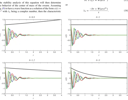
Therefore, knowing properties of the Lambert function, one can analyze the solution of Eq. (16) of the characteristic Eq. (10) and extract stability criteria that are primarily defined as Re[λk]<0 for allλk. As a multivalued function, the branches or the set of Lambert functions are denoted

Wk(z) with k∈Z. For a given triplet, (b,a,τ), the set of solutions in Eq. (16) admits a clear leading eigenvalue, the rightmost eigenvalue. The value of this rightmost eigenvalue, which is given byλ0, by conjecture determines the stability; i.e., Re[λ₀]<0 implies the center of mass will converge. Figure3 illustrates a surface (a=1) with the vertical axes corresponding to the real part of the rightmost eigenvalue of the system and the horizontal axis corresponding to the parameter

b and the delay τ. This illustrates the stable and unstable regions of the swarm, that is, when the center of mass stops and when it diverges rapidly. The eigenmodes for a subset of these values are also illustrated in Fig.4. This indicates that, in all cases, all of the eigenmodes converge to zero except in the case of the rightmost eigenmode, which is the controlling mode. However, the rightmost eigenmode is dependent on the values of the parametersaandb, as is illustrated. The equation of the velocity of the center of mass [recallx(t)=R˙c(t)] can also be explicitly defined as a solution of the delay differential equation (DDE) (9) by

x(t)= +∞

k=−∞

Ckeλkt, (17)

where λk is defined by Eq. (16) and the coefficientsCk are dependent on the initial conditions.

III. SIMULATION AND ANALYSIS FORβ=1 It has been shown in the previous section that the TDAS term can be augmented to induce either stable (stationary), marginally stable (uniformly rotating and translating bounded velocity), or unstable (exponentially diverging velocity) swarm motion. In this section we investigate the transition of these swarm topologies to rotating swarms with a stationary center of mass due to the addition of a spring potential. It is shown that introducing a spring potential alongside the Morse potential

0 _{0.5 1}

1.5 ₂ −0.5

0 0.5

−0.2 −0.15 −0.1 −0.05 0 0.05 0.1 0.15

x

|x

ij|

U i

FIG. 5. (Color online) The potential surface as a function of agent separation and the distancexfrom the origin.

0 10 20 30 40 50

0 1 2 3 4

time |v i

|

0 20 40 60 80 100

0 0.5 1 1.5 2

time

|v i

|

(i)

(ii)

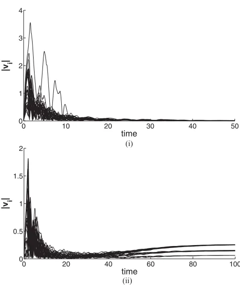
FIG. 6. The velocity magnitude history for 30 agents in the swarm: (i) a=b=1, all velocities are small and bounded, and (ii) a=1.1,b=1, velocities are bounded but their magnitudes become larger.

and used in combination with TDAS induces dynamic vortex formations about the origin. The spring potential function is purely attractive and grows linearly with the separation between each particle and the origin. Explicitly, the APF (1) is used with β =1,Ca=1,La=0.8,Cr =1,Lr =0.5, which yields the potential function surface in Fig.5. Note that forb > athe velocities will always converge to zero as in the case when the spring potential is not included. Furthermore, whenba, the velocity will diverge, and foraslightly larger thanb, the velocity will be bounded but at a larger velocity than fora =b. In other words, asb increases (abovea), the final bounded velocity will increase until it reaches a critical value, where it will diverge (escapes from the potential well). Examples of bounded velocities are illustrated in Figs.6(i) and6(ii). The two behaviors are qualitatively unchanged with each agent converging to one of three constant velocity magnitudes [this is most clearly observed in Fig.6(ii)]. From here on we assume

a=b=1, which corresponds to the marginally stable case for

β =0. Summing over all agents in Eq. (3) withβ=1 yields

i

miv˙i(t)= −

i

mivi(t)+

i

mivi(t−τ)−

i

mixi,

(18)

where _ixiis the additional component to the previous case (6) corresponding to the addition of the spring potential and

4 3 2 1 Reλk

100 50 50

(i) (ii)

100

Imλk

0.6 0.5 0.4 0.3 0.2 0.1 Reλk

40 20 20 40

Imλk

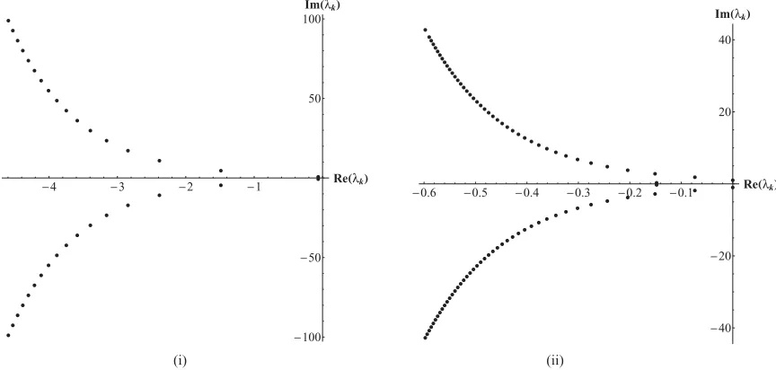
FIG. 7. Characteristic roots of Eq. (21) for (i)τ =1, where the rightmost eigenvalue has a negative real part, and (ii)τ=2π, where the two rightmost eigenvalues lie on the imaginary axis.

center of mass of the swarm can thus be expressed as

¨

Rc(t)= −R˙c(t)+R˙c(t−τ)−Rc(t); (19)

definingX=[Rc(t),R˙c(t)]T_{, this can be expressed as a linear} time delay system of the form

˙ X(t)=

_{0 1}

−1 −1

X(t)+

_{0 0}

0 1

X(t−τ). (20)

This system cannot be solved using the matrix generalization of the Lambert function as the two matricesAandBin ˙X(t)=

AX(t)+BX(t−τ) corresponding to (20) do not commute; see [28]. Therefore, the stability of the center of mass of the swarm is determined using a numerical eigenvalue based ap-proach for time-delay systems [29]. It is well known (see [29]) that as the system, shown in Eq. (20), is of the form ˙X(t)=

A0X(t)+A1X(t−τ), whereX(t)∈R2 can be expressed as X(t)= ∞_−∞Ckeλkt andA0,A1∈R2×2are real matrices and 0< τ, that the substitution of a sample solution of the form

eλkt_{v, wherev}∈_C2×1_/{₀}_{, leads to the characteristic equation}

det(λk)=0, (21)

where

(λk)=λI−A0−A1e−λkτ. (22)

The particular case when τ =1 and τ =2π is illustrated in Fig.7, where the maximum real part of all the eigenval-ues is Re(λ0)= −0.0638512 and Re(λ0)=0, respectively. Figure7illustrates that the center of mass will always stop, independently of the number of agents in the swarm, forτ =1. Figure8shows a plot of just the rightmost eigenvalue against

τ and illustrates that the center-of-mass will always stop for

τ ∈(0,2π). Moreover, each agent’s velocity has been shown to converge to a constant velocity (witha=b) and that in the pre-sense of the spring potential (in this specified range of the delay parameter) the center of mass will also stop independently of initial conditions. This implies that for random initial condi-tions the swarm must converge to a rotating motion. Figure9

illustrates convergence to the rotating (vortex) motion for a swarm of 30 agents projected on thex-yplane. However, from Fig.7(ii) (τ =2π) it can be seen that the right-most eigenvalue lies on the imaginary axis. In this case, ast → ∞, all modes converge to zero except the rightmost, and therefore the solution in the limit is a periodic motion. This periodic solution exists forτ =2nπ, wheren∈Z, and is easily shown to be

Rc(t)=R˙c(0) sint+Rc(0) cost. (23)

This periodic motion can be considered stable in that all tran-sient motion independently of initial conditions will converge to it [except for the trivial case ˙Rc(0)=Rc(0)=0]. In this case each agent winds around the origin as illustrated in Fig.10 (ii), with the periodic motion of the center of mass tracing an ellipse. If a numerical continuation of the delay parameter is extended beyondτ =2π, it is seen that the real part of the rightmost eigenvalue is always negative except at the discrete bifurcation pointsτ =2nπ. Note that the bifurcations involve two stable delay dependent steady states: an equilibrium point and a periodic orbit. However, the eigenvalues never cross the imaginary axis of the complex plane for any value of the delay

1 2 3 4 5 6 τ

0.12 0.10 0.08 0.06 0.04 0.02

Reλ0

−0.8 −0.4 0 0.4 0.8 −0.8

−0.4 0 0.4 0.8

x

y

−0.8 −0.4 0 0.4 0.8 −0.8

−0.4 0 0.4 0.8

x

y

−0.8 −0.4 0 0.4 0.8 −0.8

−0.4 0 0.4 0.8

x

y

−0.8 −0.4 0 0.4 0.8 −0.8

−0.4 0 0.4 0.8

x

y

(i) (ii)

(iii) (iv)

FIG. 9. Swarm of 30 agents forming a vortex independently of initial conditions: (i) random initial conditions, (ii)t=10, (iii)t=20, and (iv)t=40.

parameter, so it is different from the classical Hopf bifurcation reported in Schwartz and Forgotson [24].

IV. CONCLUSION

This work has investigated the combined effect of an artificial potential function (Morse potential and a spring potential) with a time-delayed autosynchronous (TDAS) term. The Morse potential is conventionally used to ensure collision avoidance and long-range attraction in swarms, while it is

shown that the TDAS term can be used to induce stationary, uniformly rotating and translating swarms or swarms with exponentially increasing translational velocity. The corre-sponding center-of-mass motion of the swarm without a spring potential is shown to be explicitly defined by a multivalued function. In the presence of a spring potential the swarm converges to a vortex formation where the center of mass is guaranteed to stop, except at discrete bifurcation points where the delay termτ =2nπ. At the discrete bifurcation points, after an initial transient, the center of mass will periodically

−2 −1 0 1 2

−2 −1.5 −1 −0.5 0 0.5 1 1.5 2

y

−0.8 −0.4 0 0.4 0.8 −0.8

−0.4 0 0.4 0.8

x x

y

(i) (ii)

trace an ellipse, whose semimajor and semiminor axes are explicitly dependent on the initial position and velocity of the center of mass. For the purpose of engineering the presented model for vortex formation has advantages over noise induced rotations as it is completely deterministic. This implies that results can be repeated and the mean field equations can be analyzed without assumptions being placed on the stochastic perturbation. In contrast to previous deterministic models for vortex formations it has a low computational requirement as the active interaction only requires that each agent is capable

of sensing its relative position within its environment without the need for any relative velocity information. This shows that it is possible to induce rotational motion with a stationary center of mass without using noise or information on the relative velocity. Therefore, these results may prove useful in controlling swarms of autonomous vehicles that posses only low computational power on board. The model could also provide a deterministic insight into swarm alignment of biological systems, such as vortex formation in schools of fish using a feedback mechanism that is a function of memory.

[1] E. Bonabeau, M. Dorigo, and G. Theraulaz,Swarm Intelligence: From Natural to Artificial Systems(Oxford University Press, New York 1999).

[2] L. Edelstein-Keshet, J. Watmough, and D. Grunbaum,J. Math. Biol.36, 515 (1998).

[3] C. Reynolds,Comput. Graphics21, 25 (1987).

[4] F. Heppner and U. Grenander, inThe Ubiquity of Chaos, edited by S. Krasner (AAAS Publications, Washington, DC, 1990), pp. 233–238.

[5] H. J. Jenson, Self-Organized Criticality: Emergent Complex Behaviour in Physical and Biological Systems (Cambridge University Press, Cambridge, 1998).

[6] A. Dussutour, V. Fourcassi, D. Helbing, and J.-L. Deneubourg,

Nature (London)428, 70 (2004).

[7] R. S. Miller and W. Stephen,Ecology47, 323 (1966).

[8] R. Gross, M. Bonani, F. Mondada, and M. Dorigo,IEEE Trans. Rob.22, 1115 (2006).

[9] W. J. Crowther, Aeronaut. J.107, 99 (2003). [10] C. R. McInnes, Aeronaut. J.107, 419 (2003).

[11] S. W. Ekanayake and P. N. Pathirana, Int. J. Adv. Rob. Syst.6, 173 (2009).

[12] D. J. Bennet and C. R. McInnes,Rob. Autonomous Syst.58, 256 (2010).

[13] A. Badawy and C. R. McInnes,J. Guidance Control. Dyn.31, 30 (2008).

[14] J. H. Reif and H. Wang,Rob. Autonomous Syst.27, 171 (1999).

[15] V. Gazi and K. M. Passino, inProceedings of the 41st IEEE Conference on Decision and Control, Vol. 3 (IEEE Press, Piscataway, NJ, 2002), pp. 2842–2847.

[16] D. E. Chang, S. C. Shadden, J. E. Marsden, and R. Olfati-Saber, inProceedings of 42nd IEEE Conference on Decision and Control, Vol. 1 (IEEE Press, Piscataway, NJ, 2003), pp. 539–543.

[17] P. Ogren, E. Fiorelli, and N. E. Leonard,IEEE Trans. Autom. Control49, 1292 (2004).

[18] D. H. Kim, H. Wang, and S. Shin,J. Intell. Rob. Syst.45, 369 (2006).

[19] D. J. Bennet, J. D. Biggs, C. McInnes, and M. Macdonald, inAutomatic Control in Aerospace, Vol. 18, Part 1, 18th IFAC Symposium on Automatic Control in Aerospace (Nara, Japan, 2010).

[20] M. H. Mabrouk and C. R. McInnes,Phys. Rev. E78, 012903 (2008).

[21] O. Khatib,Int. J. Rob. Res.5, 90 (1986).

[22] C. R. McInnes,Phys. Rev. E75, 032904 (2007).

[23] U. Erdmann, W. Ebeling, and A. S. Mikhailov,Phys. Rev. E71, 051904 (2005).

[24] E. Forgoston and I. B. Schwartz, Phys. Rev. E 77, 035203 (2008).

[25] K. Pyragas,Phys. Lett. A170, 421 (1992).

[26] P. Hovel,Control of Complex Nonlinear Systems with Delay, Springer Theses (Springer, New York, 2010).

[27] M. R. D’Orsogna, Y. L. Chuang, A. L. Bertozzi, and L. S. Chayes,Phys. Rev. Lett.96, 104302 (2006).

[28] E. Jarlebring and T. Damm,Automatica43, 2124 (2007).