Design and evaluation of multimedia extensions for the DLX architecture

Rochester Institute of Technology

RIT Scholar Works

Theses

Thesis/Dissertation Collections

6-1-1997

Design and evaluation of multimedia extensions for

the DLX architecture

Brian Hughes

Follow this and additional works at:

http://scholarworks.rit.edu/theses

This Thesis is brought to you for free and open access by the Thesis/Dissertation Collections at RIT Scholar Works. It has been accepted for inclusion

in Theses by an authorized administrator of RIT Scholar Works. For more information, please contact

[email protected]

.

Recommended Citation

DESIGN AND EVALUATION OF MULTIMEDIA EXTENSIONS

FOR THE DLX ARCHITECTURE

by

Brian W. Hughes

A thesis submitted in partial fulfillment of the requirements for the degree of

Master of Science in Computer Engineering

Department of Computer Engineering

College of Engineering

Rochester Institute of Technology

Rochester, New York

June, 1997

Approved by:

Dr. Roy Czernikowski, Professor and Department Head

Dr. Tony Chang, Professor

THESIS RELEASE PERMISSION FORM

ROCHESTER INSTITUTE OF TECHNOLOGY

COLLEGE OF ENGINEERING

Title: Design and Evaluation of Multimedia Extensions for the DLX Architecture

I, Brian W. Hughes, hereby grant permission to the Wallace

Memorial Library to reproduce my thesis in whole or in part

for non-commercial and non-profit use only.

Signature

Abstract

Multimedia

computer

architecture

extensions

for

Hennessy

and

Patterson's

DLX

architecture are

developed

following

the study

of multimedia

and

existing

multimedia architecture

Support

for

the

is

to

a

VHDL

superscalar

DLX

CPU

model as well as a

DLX

assembler.

Key

functions

used

in

digital

video

encoding

and

decoding

modified

to

use

the

extensions,

are

undertaken

using

the

VHDL

model

to

determine

the

speedup

by

the

for

these

functions. The

results of

the

simulations are used

to

calculate

the

speedup based

on

the

function speedup

and

the

fraction

the

time

that

application

spends

executing

function. It is

that the

CPU

design limits

the

performance

gain offered

by

the extensions,

concluded

that the

of

the

extensions

is

further limited

by

the

fraction

of

the

application code

that

can make use

Trademarks

MDMX

and

MIPS V

are

trademarks

of

MIPS

Technologies,

Inc.

MMX is

a

trademark

of

Intel

Corporation

PA

RISC

and

MAX-2

are

trademarks

of

Hewlett-Packard

Company

4

Multimedia

Application Performance

55

4.1

Benchmarked

Applications

56

4.2

Results

58

4.3

Target

Functions for Performance Evaluation

62

4.4

Performance

Gain

Due

to

Parallelism

for

Multimedia Applications

62

5

DLX Extension Design

66

5.1

Existing

DLX Architecture

66

5.2

Multimedia

Extensions

to

DLX

69

6

DLX Extension Implementation

78

6.1

CPU

Pipeline Structure

and

Operation

78

6.2

Extension

Implementation

81

7

System Modifications

82

7.1

DLX Assembler Modification

82

7.2

DLX

CPU

Model Modification

83

7.3

Software Modification

85

8

Extension

Performance

and

Discussion

87

8.1

Effects

of

Superscalar

Design

on

Results

87

8.2

Application

Speedup

89

8.3

Multimedia Extension

Limitations

90

9

Summary

and

Conclusion

92

References

94

A.l

Chen

IDCT

C

source

code

96

A.2

SAD

motion estimation

C

source code

(HPFastBME)

102

A.3

Unenhanced

Chen

IDCT DLX assembly

code

108

A.4

Enhanced

Chen

IDCT DLX assembly

code

123

A. 5

Unenhanced

SDS

motion estimation

DLX assembly

code

(HPFastBME)

141

A.6

Enhanced

SDS

motion estimation

DLX assembly

code

(HPFastBME)

185

Appendix B:

Application Simulation Output

224

B.l

MPEG layer

3

audio

decode

224

B.2

MPEG-2

video

decode

226

B.3

MPEG-2

video encode

228

B.4

Px64

video

decode

230

List

of

Figures

2.1

Magnitude

response of

digital

filter

5

2.2

Example

of

frame

ordering in

an

MPEG

video stream

16

2.3

MPEG

encoder

block diagram

17

2.4

MPEG decoder block diagram

19

2.5

Masking

of

frequencies due

to

movement of

threshold

of

hearing

22

2.6

Rendering

pipeline

for Gouraud

or

Phong

shading

25

2.7

Rotation

of point

p

counter-clockwise

by

angle a

28

2.8

View

volume

for

perspective

projection

31

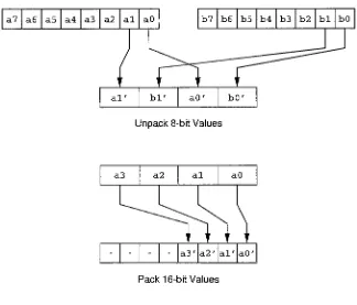
3.1

Packed Data Types

38

3.2

Operation

of

the

MAX

2

mix

instruction

40

3.3

Operation

of

the

VIS

f

pmerge

instruction

43

3.4

Operation

of

MMX

packss and punpck

instructions

47

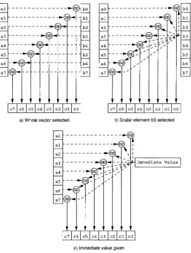
3.5

Operation

of each mode of

the

MDMX

vt-select

field

52

5.1

DLX instruction encoding formats

67

5.2

Operation

of

the

multiplication

instruction in 16-bit

elements

72

5.3

Shuffle

operation on

16-bit

elements

73

5.4

DLX instruction encoding

formats

with added

encoding

75

6.1

Pipeline

structure of superscalar

DLX

CPU

78

List

of

Tables

2.1

MPEG

standard

video

formats

15

2.2

H.261

supported

video

formats

20

2.3

Digital image

manipulation

operations

24

2.4

Outcode bits

for

6-sided

view

volume

31

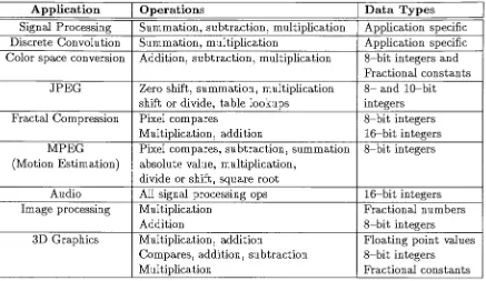
2.5

Summary

of application operation and

data

type

requirements

36

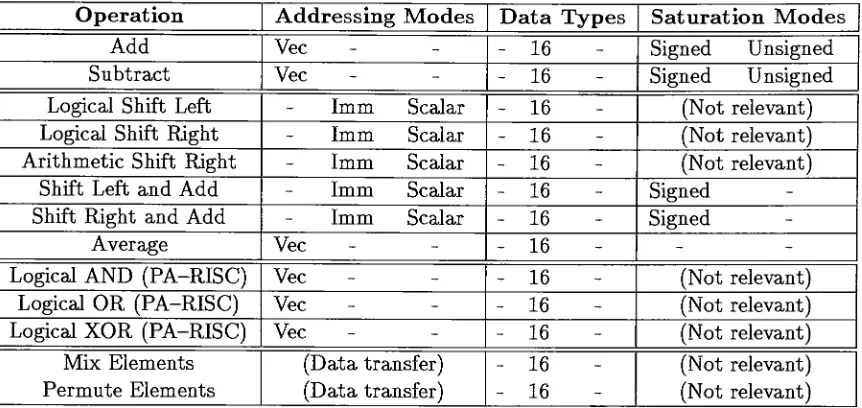
3.1

MAX-2 instructions

and supported

data

types

40

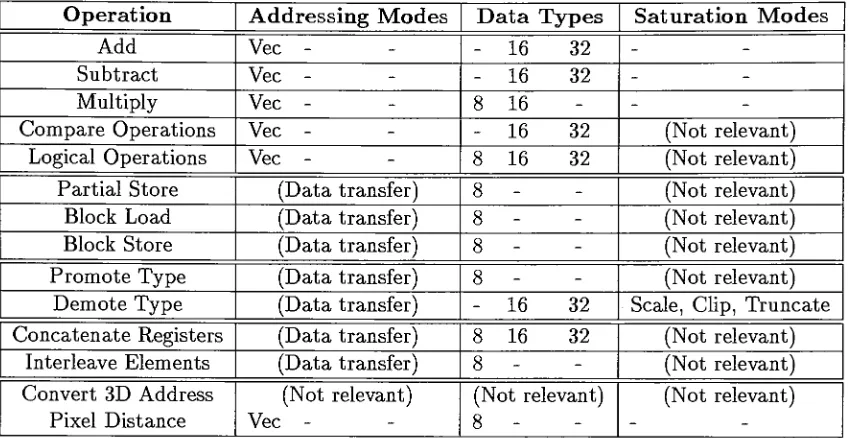
3.2

VIS

instructions

and supported

data

types

42

3.3

MMX instructions

and

data

types

supported

46

3.4

MDMX/MIPS V instructions

that

do

not use

accumulator

48

3.5

MDMX instructions

that

use additional accumulator

49

3.6

Brief

comparison

of multimedia extensions

implementations

53

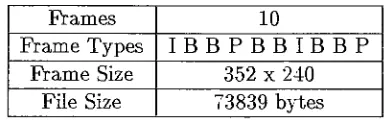
4.1

Specifications

of

decoded

MPEG

video

file

56

4.2

Specifications

of

decoded Px64/H.261

video

file

57

4.3

Specifications

of

decoded

MPEG

layer 3

audio

file

57

4.4

Five

most

costly

functions

in

MPEG

video

decoding

simulation

58

4.5

Five

most

costly

functions

in

MPEG

video

encoding

simulation

59

4.6

Five

most

costly

functions

in

Px64/H.261

video

decoding

simulation

60

4.7

Five

most

costly

functions in Px64/H.261

video

encoding

simulation

60

4.8

Five

most

costly

functions

in

MPEG

layer 3

audio

decoding

simulation

61

4.9

Code

coverage provided

by

functions

selected

for

performance evaluation

62

4.10 Application

speedup

due

to

speedup

of

Chen

DCT

and

Chen

IDCT

code

64

4.11 Application

speedup

due

to

speedup

of motion

estimation

code

64

4.12 Total

estimated

speedup

for

target

applications

65

5.2

Supported ALU

operations

in DLX

68

5.3

DLX

multimedia extension

instructions

71

5.4

DLX

main opcodes

74

5.5

DLX

SPECIAL

functions

(main

opcode

S00)

74

5.6

DLX

FPARITH

functions

(main

opcode

$01)

74

5.7

DLX

main opcodes with multimedia extensions

76

5.8

DLX

MULTIMEDIA

functions

76

5.9

DLX

M-TYPE

functions

76

7.1

Original DLX internal

floating

point

function

codes

(6-bit)

84

7.2

DLX internal

floating

point

function

codes with extensions

(7-bit)

85

8.1

Simulation

results

for

target

functions

87

Glossary

CCF

CCIR

601

CIF

DCC

DCT

Differential PCM

EDTV

JPEG

H.261

HDTV

Cross Correlation Function

used

for

MPEG

motion estimation

One

of

4

video

formats

supported

by

the

MPEG-2

video

com

pression

standard;

calls

for

a resolution of

720

X

486

at

30 Hz

and

requires

5-10 Mbps

of

signal

bandwidth

One

of

2

video

formats

supported

by

the

H.261

video compression

standard;

calls

for

a resolution of

352

X

288

Digital Compact Cassette

Discrete

Cosine Transform

used

by

the

JPEG

still

image

com

pression standard and

MPEG

video compression

for

coding

Digital coding

technique

in

which

the

differences between

succes

sive samples are encoded

using PCM

One

of

4

video

formats

supported

by

the

MPEG-2

video

com

pression

standard;

calls

for

a resolution of

960

X

486

at

30

Hz

and

requires

715 Mbps

of signal

bandwidth

Lossy

still

image

compression standard

Video

compression

standard

intended

for

video

conferencing;

sup

ports

CIF

and

QCIF

video

formats

One

of

4

video

formats

supported

by

the

MPEG-2

video

com

pression

standard;

calls

for

a resolution of

1920

X

1080

at

30 Hz

IDCT

ISDN

MAD

MAX-1

MAX-2

MCU

MDMX

MMX

MPEG-1

MPEG-2

MPEG^t

MSD

PCM

Px64

QCIF

The Inverse Discrete

Cosine

Transform

used

by

the

JPEG

still

image

compression

standard

and

MPEG

video

compression

for

decoding

Integrated

Services

Digital Network

Mean

Absolute

Difference

function

used

in

MPEG

motion

estimation

First-generation

of multimedia

extensions

for

Hewlett-Packard's

PA-RISC

architecture

Second-generation

of

multimedia

extensions

for

Hewlett-Packard's

PA-RISC

architecture;

a superset of

MAX-1

Minimal

Coded

Unit

MIPS Digital Media Extensions

for

the

MIPS RISC

architecture

Intel's

multimedia extensions

for

the

Intel

architecture

Video

compression

standard

supporting

only

the

SIF

video

format

Video

compression standard

supporting

higher-bandwidth

video

formats

including

HDTV

Video

compression standard

targeting

applications

allowing

low-resolution

images

and slow

frame

rates

Mean

Squared

Difference

function

used

for MPEG

motion

estimation

Pulse

Code

Modulation;

a

digital

coding

technique.

Colloquial

name

for H.261

Quarter CIF:

one

of

2

video

formats

supported

by

the

H.261

RGB

SIF

SAD

SDS

VIS

YCbCr

YUV

The

Red/Green/Blue

color

space

used

by

graphics

display

hardware

Lowest-resolution

video

format

supported

by

MPEG-2

and

the

only

video

format

supported

by

MPEG

1;

calls

for

a resolution

of

352

X

240

at

30 Hz

and requires a

bandwidth

of

1.2-3 Mbps

Sum

of

Absolute Differences

cost

function

used

for MPEG

motion

estimation

Sum

of

Differences Squared

cost

function

used

for MPEG

motion

estimation

Visual Instruction Set: Sun

multimedia extensions

for

the

SPARC

architecture

An

alternate

color

space

used

for digital image

representation.

Based

on

the

YUV

color

space,

with with

U

and

V

components

scaled and shifted so

they

are

always

between 0

and

1.

An

alternate

color

space

used

for digital

image

representation

comprised of a

luminance

channel

(Y)

and

two

chrominance chan

1

Introduction

Multimedia

applications

have

placed new

demands

on

both

personal computers and work

stations,

requiring

them to

process

large

amounts of

data

in

a

variety

of

formats.

Typ

ical

multimedia

areas

include

voice, audio,

still

and

animated

graphics,

and

full

motion

video

[LS96]. Some

issues

when

dealing

with

these types

of

data

are media

synchronization,

storage requirements

for

multimedia

data,

and

the transmission

of multimedia

data between

machines on a network.

Typically,

the

amount of multimedia

data

that

needs

to

be

available

to

provide

any

amount of meaningful content with good

quality

is

large. An

example

is

given

in

[FSZ95]

for

a multimedia

encyclopedia comprised of

500,000

pages of

text,

3,000

color

pictures,

500

maps,

60

minutes of stereo

sound,

30

animations,

and

50 digitized

movies

(1

minute

each);

this

particular encyclopedia

would require

111.1

GB

of storage

capacity if

each element

was

stored

in its

native

format.

In

addition

to

storage

capacity,

video and audio

streams

require

a

specific

bandwidth

between

the

source and

the

viewer

to

be

played at real-time rates.

As

a

result,

much effort

has been

put

into

the

development

of compression and

decompression

technologies

and

standards such

as

JPEG

and

MPEG

to

provide a

means

to

reduce

the

amount of

storage required

for

multimedia

data.

Also

characteristic

to

multimedia systems

is

the

need

to

process

this

data. For example,

algorithms

may

be

applied

to

an

image

or series of

images in

a video

to

enhance

their

quality

or scale

them to

fit

in

a window.

The

manipulation

of audio

data

may

require

the

mixing

of

two

or more

audio

streams.

The

Intel Media Benchmark

[Int96],

designed

to

evaluate

performance

of

multimedia personal

computers, includes

sections

which

brighten

an

image

and

blend

two

stereo audio streams

together.

To

speed

the

execution

of multimedia

data

compression

and

decompression

algorithms

their

CPU

architectures

to

better

support

multimedia applications

[LS96]. All

extensions

focus

on

SIMD

parallelism

on small

data

types,

and support

this

parallelism

by

"packing"

a number

of small

data

elements

into

a

single,

wide

register

and

performing

operations

in

them

in

parallel.

The

goal

of

this thesis

will

be

to

add such support

to

Hennessy

and

Patterson's DLX

architecture

[HP96]

and

evaluate

the

performance

gain

offered

by

such

extensions

through

the

simulation of real multimedia applications on a

VHDL

model of a

DLX

CPU,

described in

[Fer96].

An

outline of

this

report

follows.

First,

sections

2

and

3

will

discuss

typical

multimedia applications

and

existing

architec

ture

extensions

designed

to

increase

their performance,

respectively.

Section 5

will propose

a set

of extensions

to the

DLX

architecture

based

on

the

examination of multimedia

appli

cations

in

section

3

and executions profiles

of multimedia applications

discussed in

section

4.

The implementation

of

the

DLX

multimedia extensions

in

a

DLX

CPU

will

be

considered

in

section

6,

with

the

required

VHDL

model

and

assembler

modifications

discussed

in 7.

Finally,

the

changes

in

performance

due

to

the

extensions and an analysis of

the

results will

2

Multimedia Applications

and

Algorithms

This

section will

discuss

compression,

decompression,

and

processing

algorithms

for

images,

video,

and audio

data

followed

by

a

discussion

of

the

computations required

for

3D

graphics

rendering.

Of interest

to this

work are

the

computational requirements required

to

support

these

applications.

The

material presented

in

this

section

is

not meant

to

be

complete and

all

issues involved in

the

design

and

implementation

of

applications

described

in

this

section

will not

be dealt

with,

but

some

background

theory

will

be

given

to

support claims made

about computational

and

storage requirements.

2.1

Digital Signal Transforms

and

Filtering

Digital

signal

transformation

and

filtering

are used

in

many

multimedia

applications,

serv

ing

to

process

digital images

[FvDFH96]

and

divide

an

audio

signal

into

subbands

for

compression

[Poh91].

Digital

signal

processing is

discussed

in

[Poh91].

The

process

of

filtering,

whether

in

the

digital

or

analog

domain,

aims

to

eliminate

certain

frequency

components

from

a signal while

retaining

others.

A

number

of

different

types

of general

filters

exist,

including

Low-pass

filters

which pass

low

frequencies

while

removing

high

frequencies,

High-pass

filters

which

pass

high frequencies

while

removing

low frequencies

Band-pass

filters

which

allow

a

range

of

frequencies

to

pass

while

eliminating

all

others,

and

Notch

filters

which suppress a range of

frequencies

and allow all

others

to

pass.

The

concept

of signals

in

the

frequency

domain

as

well

as

sampling

theory

are

both

important

to the

understanding

of

digital filters. The

reader

is

directed

to

[Poh91]

for

more

The

z-transform

is

central

to the

design

and

analysis

of

digital

filters,

as

digital

filter

transfer

functions

are

described

in

terms

of

the

digital

variable

z.

The

z-transform

is

described

mathematically

as

[Poh91]

+00

(2.1)

X(z)=

J2

7l= OO

and,

as

shown,

converts

a

discrete

time

signal

into

the

digital

frequency

domain. In

engi

neering,

a

one-sided 2-transform

is

typically

used

which

involves

the

summation

from

0

to

00,

rather

than

to

00 as shown above

[Poh91].

A

transfer

function,

as

a

function

of

z,

describes

a

digital filter.

In its

most

general

form,

the transfer

function

of a

digital filter is

[Poh91]

(2-2)

E[z)

,

^^

1

+

The

numerator of

the transfer

function

has M

roots,

called

zeros,

while

the

denominator

has

N

roots,

called poles.

The

locations

of

the

roots and poles

in

the

digital

frequency

plane

describe

the

frequency

response of

the

digital

filter,

which can

be determined

graphically

by

tracing

a path

along

a unit circle

in

the

z-plane and

noting

the

distance

of

the

point

from

poles and

zeros

to

determine

the

magnitude of

the response,

while

the

angle

from horizontal

made with each pole and zero

determines

the

phase response.

Specifically,

the

magnitude

response at point

A

in

the

unit circle

is

given

as

(2-3)

\H{z)\

"fl

l^-g

1

lj=i

I--

-HI

where

Z{

is

the

zero and

Pj

is

the

for

point

A

is

(2.4)

M

N

8=0

j=0

where

^i

is

the

angle

from

the

zero and

$;

is

the

angle

from

the

pole.

An

example

for

the

filter

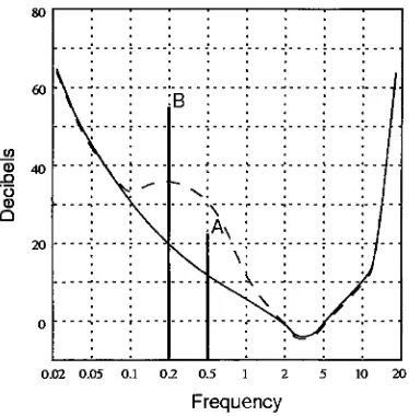
(2.5)

H(z)

ill

2z

with a zero at

and a pole at

0 is

shown

in

figure

2.1

[Poh91].

|Y(z)|

Re(z)

Figure 2.1:

Magnitude

response

of

digital filter

Given

a

digital filter

transfer

function,

an

inverse

z-transform

can

be

applied

to

it

to

yield a

difference

equation of

the

form

M

N

(2.6)

y(n)

X)a^(n

*)

J2bty(n

-{)

Equations

of

this

form

must

be

processed

by

a

computer

system

to

implement

a

digital

filter.

Note

that

as

the

number of poles and zeros

increases,

the

computational

complexity

increases

but is

still

limited

to

multiplication and addition operations.

Alternately,

[FvDFH96]

approaches

digital

filtering

through

convolution.

The Discrete

Fourier

Transform

(DFT)

can

be

used

to

convert a

digital

signal

into

the

frequency domain,

and multiplication can

be

used

to

remove unwanted

frequencies,

and a subsequent conversion

back

to the

spatial or

temporal

domain

produces

the

desired

result.

For

example, to

remove

all

frequencies

above

frequency k,

convert

to the

frequency

domain

and

multiply

by

the

pulse

function:

1,

when

k

<

u

<

k,

(2.7)

S(u)

0

elsewhere

As

discussed in

[FvDFH96],

multiplication

in

the

frequency

domain

is identical

to

con

volution

in

the time

domain,

so

the

process

described

above can

be

replaced

by

a single

convolution.

A

convolution

is

defined

as

[FvDFH96]

/oo

f(r)g(x

-r)dr

-oo

A discrete

convolution

is

defined

as

[Poh91]

CO

(2.9)

h(n)=

Y,

x(k)h{n-k)

k=oo

Convolution

using

a pulse

function

as

defined

in

equation

2.7 is

known

as

box filtering. As

with

the

processing

of

difference equations,

a

number

of

multiplications

and

additions

are

required

to

evaluate

the

output of a

digital filter

using

a

convolution.

In

either

case,

the

2.2

Color Spaces

and

Color Space Conversion

Of

importance

to

image/video

compression and

processing

algorithms

is

the

color space of

an

image.

Each

pixel

in

an

image is

defined

by

one of more color elements.

A

pixel

in

a

24-bit

color

image,

for

example,

will

have

an

8-bit

element

for

each of

its

red,

green,

and

blue

component.

This is

known

as

the

RGB

color

space.

As discussed in

[FSZ95],

it is

more natural

for

compression algorithms

and,

as

discussed

in

[Int96]

some

image processing

algorithms, to

operate

in

the

YUV

color space

in

which

the

Y,

or

luminance,

component

specifies

the

brightness

of

the

pixel and alone can

produce

a

greyscale

image.

The

U

and

V,

or

chrominance,

components are used

to

add color

to the

image.

RGB

to

YUV

conversion

is

defined

by

the

CCIR

601

standard as

[FSZ95]

(2.10)

Y

0.299i? + 0.587G-r-0.114fi

(2.11)

U

0.564(5

-Y)

(2.12)

V

0.713(J?-Y)

Note

that

equation

2.10 is

a weighted

average of

the

R,

G,

and

B

components

of

the

image

and will result

in

a value

requiring

the

same number of

bits

as

the

inputs

components.

Equations 2.11

and

2.12

will require

the

signed

computation

(pixel

components

are

typically

unsigned)

and

may

require additional

bits

for intermediate

and

final

values.

The

conversion

of a pixel with

B

0

and

Y

255

will result

in

V

-181.82,

for

example,

which cannot

be

represented

in 8 bits.

R

G

B

Y

+

TT

+

4

2

2

B

U

2

R-Y

(2.13)

(2.14)

(2.15)

V

2

The

inaccuracy

introduced

by

this

formulation is

apparent

by

comparing it

to the

CCIR

standard

definition in

equations

2.10, 2.11,

and

2.12.

Fast

multiply

of

multiply-accumulate

operations,

such

as

are supported

by

the

PA-RISC

2.0

architecture

[Lee96],

Intel's MMX

[P

WW97],

and

MIPS

MDMX

[MIP96b]

can enable

the

use

of more accurate

RGB

to

YUV

color space conversions.

Also

used

in image

compression

and

processing

algorithms

is

the

YCbCr

color space

[FSZ95]

It is

similar

to the

YUV

color

space,

but

scales

and zero-shifts

the

U

and

V

components

so

that

they

are always

between

0

and

1.

To

convert

the

U

and

V

components of

the

YUV

color space

to the

Cb

and

Cr

components of

the

YCbCr

color

space, the

following

equations

are used

[FSZ95].

(2.16)

Cb=j

+ 0.5

(2.17)

Cr

Ye

+ -5

2.3

Still Image Compression

Still

image

compression

techniques

aim

to

compress

still

images and,

addition

to

this,

are

used

to

compress video at

the

intra-frame

level.

Compression

techniques

can

be

classified

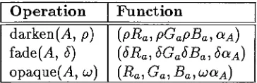
into

two

categories:

lossless

and

lossy

[FSZ95]

will

provide

an exact

duplicate

of

the

original

image

after

decompression,

while

lossy

or

noisy

techniques

will

not.

A

lossy

compression

algorithm

allows

the tradeoff

of signal

quality

for

compression

ratio,

and

can

produce

compressed

images

which

are

discernible

from

the

original when

operating

with a

high

quality

setting.

2.3.1

The

JPEG

Image Compression Algorithm

JPEG

is

a still

image

compression algorithm

designed

to

work on

full-color

images,

and

is

discussed

thoroughly

in

Chapter 5

of

[FSZ95].

The

JPEG

standard

defines four

modes of

operation,

1. Sequential DCT-based

encoding

in

which

each

image

component

(each

component

in

the

color

space)

is

encoded

in

a single

left-to-right,

top-to-bottom

scan

and

the

discrete

cosine

transform

(DCT)

is

used

to

convert

the

image

from

the

spatial

(image)

domain

to the

frequency domain,

2.

Progressive

DCT-based

encoding,

another method

using

the

discrete

cosine

transform

but in

which

the

image is

encoded

in

multiple

scans,

each scan

increasing

the

image

resolution and

therefore the

image

quality,

3.

Lossless

encoding

which uses no

lossy

transformations

and

guarantees

an exact repro

duction

of

the

original

image

upon

decompression,

and

4. Hierarchical encoding in

which

the

image is

encoded at

multiple resolutions.

For

multimedia

applications,

lossy

encoding is usually

acceptable and

sometimes

neces

sary

as

it

provides

the

highest

compression ratios.

The

following

sequence

of

steps

is

used

to

encode

an

ra-bit-per-pixel

greyscale

image

using

the

sequential

DCT-based

encoding

technique.

1.

the

input

values

are

shifted

from

the

range

0

to

-1

to

the

range

to

2.

the

resulting

values are

grouped

into 8x8

blocks,

3.

the

discrete

cosine

transform

is

used

to

convert each

block

of

the

input

data

from

the

image

domain

to the

frequency domain,

4.

the

resulting DCT

coefficients are quantized

using

a quantization

table,

reducing

the

amplitude

of

the

DCT

coefficients

and

producing

more

zero-valued

coefficients

to

increase

the

effectiveness of

the entropy encoding,

5.

the

quantized

coefficients are reordered such

that the

lowest-frequency

coefficients are

first,

6.

the

ordered coefficients are encoded

using

entropy

encoding.

In

[FSZ95],

the

DCT

for

an

8

x

8

block

is

defined

as

follows.

,,. ,_,.

,

C(u) C(v)

J^ J^

(2x

+ 1)utt

(2y+lW

(2.18)

F(u,v)

^ULJ2Ylf(x>y)cos-

16

2;=0 j/=0

where

C(u)

75

ifw

>

1

if

u>0

and

f(x,

y) is

the

an

8

x

8

block from

the

input

image. The

DCT

outputs

an

8

x

8

block

of

DCT

coefficients

in

which

F(0, 0)

is

called

the

"DC

and

the

remaining

63

values

are called

"AC

coefficients"

.

The

number

of

bits

required

to

store

a

single coefficient

can

be

more

than those

required

to

store

the

input

pixel values.

In

[FSZ95],

it is

pointed out

that

for

a greyscale

image

with

input

pixels

in

the

range

[-128,

127]

(8

bits

per

pixel),

the

pixel

of storage.

This

is

significant

to the

design

of

multimedia

hardware because

simple

8-bit

data

types

cannot support a

DCT

on

8-bit

values

to

full

accuracy.

Quantization,

described

in

both

[FSZ95]

and

[Poh91],

is

given

as

(2.19)

Fq(u,v)

Round

F(u,

v)

Q(u,v)

where

Q(u,v)

is

an

entry in

the

quantization

table

and

is

between

1

and

255,

an

8-bit

unsigned

value.

Quantization

is

the

simplest

form

of

lossy

compression

[Poh91].

Due

the the similarity

of

DC

coefficients

between

different

blocks,

predicative

coding

can

be

used

to

encode

the

DC

coefficients.

That

is,

the

first

DC

coefficient

is

coded

directly,

and

subsequent

DC

coefficients are each subtracted

from

the

previous

and

the

result

is encoded,

usually

requiring fewer

bits

for

representation

than

direct

coding.

Many

encoding

schemes can

be

used

to

perform

the

entropy encoding

of

the

quantized

DCT

coefficients

in

the

last step

of

the

JPEG

algorithm.

In

[FSZ95],

Huffman coding is

used and

it is

noted

that

arithmetic

coding may

also

be

used.

Both Huffman coding

and

arithmetic

coding

are presented

in

Chapter

8

of

[Poh91].

To

perform

Huffman coding, input

sequences

are

first divided

into intermediate

se

quences

consisting

of

any

number of zeros

followed

by

a non-zero value.

The

zero

portion

of

the

sequence

and

the

number

of

bits

used

to

represent

the

non-zero

portion

of

the

se

quence are encoded

in

a

(RUNLENGTH, SIZE)

pair where

RUNLENGTH

is

the

number

of

zeros

and

SIZE

is

the

number of

bits

used

to

represent

the

non-zero value.

Next,

the

non-zero

value

is

encoded

in

a single

(AMPLITUDE)

symbol which

is

SIZE bits

in

length.

The

number of

bits

allocated

for RUNLENGTH

and

SIZE

is

fixed

at

four,

and

the

pair

(15,

0)

is

used

to

represent

a

RUNLENGTH

of

16.

To

encode

RUNLENGTHs

greater

than

16,

a

number of

(15, 0)

pairs can

be

used,

each

representing

an additional

16 zeros,

followed

by

The

(RUNLENGTH, SIZE)

pairs

formed

above

are

then

encoded

in

binary

using

a

variable

length

code

from

a

Huffman

table,

and

the

(AMPLITUDE)

symbols are encoded

using

a variable

length

integer.

JPEG

decoding

performs

the

inverse

of

the above,

performing

entropy

decoding

followed

by dequantizing,

the

inverse

discrete

cosine

transform

or

IDCT,

and zero-shifting.

Dequan-tizing

involves simply multiplying

the

quantized

value

by

its corresponding

entry

in

the

quantization

table.

The IDCT

for

an

8

x

8 image block

is

defined

as

(2.20)

f{x,y)

-J2Y,C(u)C(v)F(u>v)cos-I^^cos

i6

where

C(u)

is

defined

as

above,

and

F(u,

v)

is

the

DCT

coefficient at

(m,

v).

JPEG

coding

of color

images is

similar

to

JPEG

for

greyscale

images

but

will

typically

employ

color space conversion and must account

for

all color segments of

the

image.

Non-interleaved

data ordering involves encoding

each component

separately in

a

left-to-right,

top

to-bottom

pass.

Interleaved ordering

requires

the

formation

of minimal

coded

units

(MCUs)

which are comprised of a number of elements

from

each color segment.

When

all

segments are of

the

same

resolution,

an

MCU

consists of one element

from

each segment.

If different

resolutions

are

used,

those

elements

containing

more

data

will contribute more

elements

to the

MCU

such

that the

final

interleaved

data

stream will

have

whole number

of

MCUs,

all

with

the

same

length.

In

either

case,

the

computational

requirements

for

color

JPEG

coding

and

decoding

increases

by

a

factor dependent

on

the

number

of

color

components

present

in

the

image

and

their

resolution.

Typically,

each

image

component

is

2.3.2

Fractal

compression of still

images

While

not supported

by

a

standard,

fractal

compression

is

relevant

to

multimedia

due

to

its

ability

to

overcome

the

resolution

dependence

of

JPEG

and

its fast decompression

times.

Fractal

compression

is

discussed

in

[FSZ95].

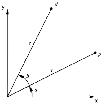
Fractal

compression uses affine

transformations,

which are combinations of

scale, rotate,

skew,

and

translate operations, to map

parts of an

image

to

other parts of

that

same

image.

Affine

transformations

are

discussed

in

both

[FSZ95]

and

[FvDFH96],

and can

be

expressed

in

the

form

(2.21)

xnew

ax

+

by

+

c

(2.22)

ynew

dx + ey +

f

where

(x,y)

is

an

input

coordinate,

and

a,b,c,d,e

and

/

are

the

coefficients

of

the

affine

transformation.

A

simple

scale

and

translate

can

be

realized

with coefficients

a

Sx,

b

0,

c

Tx,

d

0,

e

Sy,

f

Ty

where

Sx

and

Sy

are

the

amount

to

scale x and

y

by,

respectively,

and

Tx

and

Ty

are

amounts

to translate

x and

y

by,

respectively.

More

complex

affine

transformation

are required

for

computer

graphics

applications and will

be discussed

in

section

2.7.1.

Note

that the

data

types

and

sizes

required

for

affine

transformations

are

dependent

on

the

size of

the

image,

and

that

signed

numbers

are

not

required

if

the

origin

is

placed

at

the

corner of

the

image.

Given

this,

8-bits

can

accommodate

256

X

256

pixel

images,

and

16-bits

can

accommodate

images 64A;

pixels square.

Fractal

compression

methods work

to

identify

self-similar regions of an

input image. To

perform

the compression, the

image is

first divided

into

domain

regions and

range

regions,

which can

be

of

arbitrary

shape,

cannot

overlap,

and must

cover

the

entire

image.

Next,

a

set of affine

transformations

are

defined

to

be

used

during

the

compression

process.

The list

is

applied

and

the

result

compared with each range region

in

the

image. For

each

domain

block,

a range

block

that

matches

the

domain block

as

closely

as possible

is

found

and

the

coefficients

for

the

affine

transformation

are saved

in

the

output

file.

To

reconstruct

the

image,

each

domain

block is

replaced with

the transformed

data from

the

matching

range

block.

Because

the

fractal-compressed

image

file

is,

in

essence,

an equation

defining

the

image,

the

image

can

be

reconstructed at

any

resolution without

loss

of quality.

2.4

Digital Video Compression

A digital

video

is

a series

of

images intended

to

be

played

back

at a

given

frame

rate.

Dig

ital

video compounds

the

storage space requirement created

by

still

images

on multimedia

systems,

and

additionally imposes bandwidth

requirements on

the

digital

video playback

system.

The

bandwidth

required

to play

back

a

digital

video

increases

with

the

frame

resolution,

image quality,

and playback rate.

To

date,

software-only

solutions

for

real-time

video

decompression

exist

[Lee96],

but

require multimedia enhanced

CPUs

such as

the

one we are

designing.

Software-only

video

compression

systems

exist,

but

because

of

the

computational

complexity involved

they

require

hand-coded

assembly

language

tailored to the

architecture of

the

CPU

they

run

on

[Kas96].

2.4.1

MPEG Compression

of

Digital Video

The

MPEG

standard,

discussed in

[FSZ95],

covers

digital

video,

digital

audio,

and synchro

nization

of

the two.

This

section will

focus

on

the

digital

video portion

of

the

standard.

The

MPEG

standard

specifies

a

number

of

different

video

resolutions,

as

shown

in

table

2.1;

support

for

these

formats

varies

with

the

phase of

the

standard.

MPEG-1,

for

MPEG-4,

unlike

MPEG-1

and

MPEG-2,

targets

video

telephony

and other applications

in

which small

frames

and

low

refresh rates are

acceptable, this

allowing it

to specify

bandwidth

requirements of

only 9

to

40 kbps.

Specification

Resolution

Frame Rate

Required BPS

SIF

352

x

240

30 Hz

1.2-3 Mbps

CCIR

601

720

x

486

30 Hz

5-10 Mbps

EDTV

960

x

486

30 Hz

7-15 Mbps

HDTV

1920

x

1080

30 Hz

20-40 Mbps

Table 2.1:

MPEG

standard video

formats

The MPEG

standard

frame

types

and

definitions

are given

in

both

[CK96]

and

[FSZ95].

In MPEG

compression, three

frame

types

are used

1.

I

frames

are

full images

compressed with a

DCT-based

technique

such as

JPEG,

2.

P

frames,

or

predicted

frames,

are

based

on

the

most

recent

I

of

P

frame

and

are

encoded

using

forward

prediction

in

which

differences from

the

reference

frame

are

encoded,

not

the

whole

frame,

3.

B

frames,

or

bidirectional

frames,

can

be

encoded

using

forward

prediction

as

in P

frames,

backward

prediction

from

the

next

I

or

P

frame,

or

bidirectional

interpolation

from

an

I

or

P

frame before

it

and

an

I

or

P

frame

after

it.

There is

a

trade-off

in

the

frame

types

used

between frame

accuracy

and

compression

ratio.

I

frames

support

the

greatest amount

of

accuracy,

but

offer

the

lowest

compression

ratios,

while

P

frames

decrease

the

accuracy

and

increase

the

compression

ratio,

and

B

frames

offer

little

accuracy

and

very

high

compression ratios.

Due

to the

nature of

B

frames,

the

storage or

transmission

order of

MPEG frames

cannot

transmission

order and

viewing

order.

Note

that the

P

frame

transmitted

second

is

viewed

fourth,

as

it is

required

to

produce

the

B

frames

viewed

as

frames

2

and

3.

The

pattern

repeats

for

the

rest of

the

MPEG

video stream.

Transmit

Order

I

P

B

B

P

B

B

P

B

B

P

B

B

I

B

B

Frame Number

1

4

2

3

7

5

6

10

8

9

13

11

12

16

14

15

View

Order

I

B

B

P

B

B

P

B

B

P

B

B

P

B

B

I

Frame Number

1

2

3

4

5

6

7

8

9

10

11

12

13

14

15

16

Figure 2.2: Example

of

frame ordering in

an

MPEG

video stream

The MPEG

compression

algorithm works

to

compress single

I

frames

and perform motion

estimation

between I

frames,

P

frames,

and

B

frames

for

inter

frame

compression.

JPEG

compression

is

typically

used

for

the

compression

of single

frames

and

was

discussed

in

section

2.3.1.

Here

we will

focus

on

the

computations

required

to

perform motion

estimation

for

inter-frame

compression.

A

block diagram

of an

MPEG

encoder,

from

[FSZ95],

is

shown

in

figure

2.3.

The figure

shows

the

compression of

I

frames

being

identical

to

color

image

compression with

JPEG.

The

production

of

B

and

P

frames

involves calculating

the

pixel

difference between

the

current

frame

and

a reference

frame

and

performing

motion

estimation

between

the two

frames.

The

goal

of motion

estimation

is

to

produce

a

vector

representing

the

motion

of a pixel

block from

one

frame

to the

next.

To

accomplish

this,

the

contents

of a

source

block

are

compared

with other

blocks

within

a

specific search region

by

evaluating

a

function

whose

output

is indicative

of

the

similarity

between

the two

blocks.

As

discussed

in

[FSZ95],

the

MPEG

standard

does

not

specify

a

block

size or a

search

region,

but

typically

16

X

16

blocks

Input

Image

RGB

to

YUV

Conversion

*-T

DCT

J*\

Quantization}

Encoder

Entropy

Input

Image

RGB

to

YUV

Conversion

Tiror

Terms

Reference

Frame

-Cdct>

Motion

Estimation

y

I Rame

1

Entropy

Encoder

>

P/B Frame

Figure 2.3:

MPEG

encoder

block

diagram

defines

several

functions

for

use

in block

comparison.

The Mean Absolute Difference function is defined

as

follows

(2.23)

MAD{dx,dy)

J2 E

\F{i,j)-G(i

+

dx,j

+

dy)\

mn

-m

'= J=

where

F(i,j)

is

a

(m

X

n) block in

the

current

frame,

G(i,j)

is

the

block

being

compared

against

in

another

frame,

and

[dx,

dy)

is

the

search

location. To

search a

28

X

28

pixel

block,

dx

and

dy

must

vary

by

6 in both

the

positive and negative

direction.

The

magnitude of

the

maximum

number

of pixels

that the

search

location is

moved

from

the

source

block

location is

p,

and

in

most

cases, p

6

[FSZ95].

Removing

the

division

by

the

constant

in

the

Mean

Absolute

Difference

equation

result

in

the

Sum

of

Absolute Differences

function

implemented

by

Sun

VIS

pdist

instruction,

discussed in both

[TONH96]

and

[MIP96b].

The Mean Squared Difference function is

a more

accurate

measure of pixel

distance

[FSZ95,

MIP96b]

but involves

a squared

term

to

remove

the

sign

of

the

difference,

rather

than

the

ab

Difference function is defined

as

Tl T71

2 2

(2.24)

MSB(dx,

dy)

(i?(j,

j)

-G(i +

dx,j

+

" ._"> "

2 2

As

above,

the

division

by

the

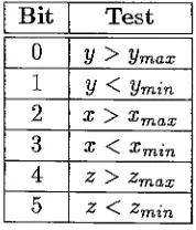
constant

can

be

removed

from

the

MSD function

and

results

in

the

Sum

of

Differences

Squared,

discussed

in

[MIP96b]

and

implemented

in

the

MIPS

MDMX instruction

set.

Lastly,

the

correlation

function

is

defined

as

E; E,

F(i,

j)G(i

+

dx,j

+

dy)

(2.25)

CCF(/z,

dy)

^l

^3

\

J>

V

y)

r

(E,EJi?2(i,j))^(EIE,G2(i-r-dx,j

+

dy))2

The

cross-correlation

function

as

defined

above

is very

expensive

to

implement,

and

is

not

commonly

used

because

of

this.

Also

of

importance

to

MPEG

compression

implementations is

the

search pattern used

to

find

the

destination

block

of

the

motion vector.

[FSZ95]

presents several approaches

to

this problem,

including

Exhaustive search,

which

simply

compares

the

source

block

against all

blocks

in

the

search

area;

Three-step

search which

computes

the

distance

of

the

center

and

at

the

eight

sur

rounding

search

locations

in

the

search

area, using

the

closest match as

the

center of

the

search

area

for

the

next

stage,

and so on.

Other

search

patterns

include

the

Conjugate Direction Search

and

the

2D

Logarithmic

Search.

As

search

patterns

do

not

have

an

affect

on

architecture

at

the

instruction

level

(although

they

may

have

an

effect on

the

cache),

so

they

will

not

be

considered

further

Input

Image

Bit

Stream

Decoder

Dequantizer

Previous

Picture

Future

Picture

IDCT

Motion

Compensation

r\.

Output

Image

Figure

2.4:

MPEG decoder block diagram

A block diagram

of

an

MPEG

decoder,

from

[FSZ95],

is

shown

in figure 2.4. For I

frames,

the

decoder

simply

dequantizes

the

data

and performs an

inverse

discrete

cosine

transform

on

the

result

to

produce

the

output

frame.

If

the

frame

will

be

used

for future

motion

compensation

functions,

it is

stored

in

either

the

"previous

or

"future

picture"

buffer

(depending

on

the

frame

number).

P

and

B

frames

are constructed

using

data

in

the two

picture

buffers

just

described;

the

motion

compensation

unit

is

responsible

for

performing

a

translation

of a source

block along

the

motion vector

to

its

destination

when

decoding

unidirectional

predictive coded

data

(P

or

B

frames)

or

interpolating

between

the

previous and

future

pictures

with

the

motion

data

(B frame only)

2.4.2

Px64/H.261 Video

Compression

The H.261

standard

for

video

compression

targets

video

teleconferencing

applications

and

is designed

to

work

over

ISDN

networks.

It is

discussed

in

[FSZ95],

and supports

the

CIF

and

QCIF

(quarter

CIF)

video

formats

with

resolutions

shown

in

table

2.2.

Specification

Y Resolution

U

and

V

resolution

CIF

352

x

288

176

x

144

QCIF

176

x

144

88x72

Table 2.2: H.261

supported video

formats

data.

H.261

does

not,

however,

use

bidirectionally

interpolated

frames,

relying

only

on

forward

prediction

(like

MPEG P

frames)

and

basing

each new

frame

off

the

most

recently

received

frame.

Furthermore,

the

interframe coding

scheme

of

H.261,

while

still

using

motion estimation similar

to

MPEG,

is

based

on

differential

PCM,

described

in

[Poh91].

The H.261 decoder

performs

functions

similar

to

the

MPEG decoder

shown

in

figure

2.4,

but

adds a

filter

to

remove

high-frequency

noise

for

the

incoming

video stream.

2.5

Digital Audio Compression

Digital

audio compression

in

general

is

discussed

in

[Poh91],

while

[FSZ95]

briefly

describes

the

MPEG

audio compression algorithm.

The

more complex audio compression

algorithms,

including

that

of

MPEG,

involve

subband

coding

and

bit

allocation

based

on

a

psychoa-coustic model

which,

similar

to

how

JPEG

compression removes

detail

not

likely

to

be

seen,