Non-Rigid Structure from Motion

(1)

Non-Rigid Structure-from-Motion

Thesis by Suryansh Kumar

to

College of Engineering and Computer Science in partial fulfillment of the requirements

for the degree of Doctor of Philosophy

in the subject of Computer Vision

Australian National University Canberra, ACT 2601, Australia

(2)

Declaration of Originality

(3)

Copyright Declaration

The copyright of this thesis is retained with the author and is available to use under Non-Commercial, No Derivative and Creative Commons Attri-bution license. Users may distribute or copy the content presented in this Thesis on the condition that they provide proper credit to it. For any com-mercial reuse, redistribution or transmission, the user must agree to li-cense terms of this work.

(4)

Advisors: Prof. Yuchao Dai, Prof. Hongdong Li Suryansh Kumar

Non-Rigid Structure-from-Motion

Abstract

This thesis revisits a challenging classical problem in geometric computer vision known as “Non-Rigid Structure-from-Motion” (NRSfM). It is a well-known problem where the task is to recover the motion and 3D shape of a non-rigidly deforming object from image data. A reliable solution to this problem is valuable in several industrial applications such as vir-tual reality, medical surgery, moviesetc. To date, there does not exist any algorithm that can solve NRSfM for all kinds of conceivable motion. As a result, additional constraints and as-sumptions are often employed to solve NRSfM. The task is challenging due to the inherent unconstrained nature of the problem itself as many 3D varying configurations can have sim-ilar image projections. The problem becomes even more challenging if the camera is moving along with the object.

The thesis takes on a modern view to this challenging problem and proposes a few algorithms that have set a new performance benchmark to solve NRSfM. The thesis not only discusses the classical work in NRSfM but also proposes some powerful elementary modifications to it. The foundation of this thesis surpass the traditional single object NRSFM and for the first time provides an effective formulation to realize multi-body NRSfM.

Most techniques for NRSfM under factorization can only handle sparse feature correspon-dences. These sparse features are then used to construct the scene using organization of points, lines, planes or other elementary geometric primitive. Nevertheless, sparse represen-tation of the scene provides an incomplete information about the scene. This thesis goes from sparse NRSfM to dense NRSfM for a single object, and then slowly lifts the intuition to realize dense 3D reconstruction of the entire dynamic scene as a global as rigid as possible deformation problem.

(5)

Advisors: Prof. Yuchao Dai, Prof. Hongdong Li Suryansh Kumar

a wide range of scenarios.

(6)

Acknowledgments

First and foremost, I would like to thank my supervisory panel. Most Ph.D. students feel blessed to get one supportive supervisor. I hadthree!.Yuchao Dai: this thesis would not have been possible without your continuous support and guidance. Thank you for introducing me to the world of non-rigidity. Your meticulous guidance and constant effort to develop me as a researcher is a perpetual source of knowledge and inspiration. Your constant rigor when I have been sloppy, helped me to learn so, so much. Your complete faith and belief in my abilities gave me a certificate to experiment over my ideas and put it to work. Most of all, thank you for your unshakable patience, humility and providing me the freedom to explore new ideas. Hongdong Li: Where do I begin? Thank you for all those productive research discussions, hours of meeting sessions and always putting me to thinkvisually. Your ability to bring ideas from different fields of science to computer vision problems has increased my dimension of thinking, so a BIG thank you for that. Also, thank you for patiently listening to my request and always responding to my “Door knock”. Thank you for correcting my paper writing and exposing my common mistakes including paper titles and my terrible figures and, last but not the least, surviving my insufferable presentation slides.Richard Hartley: Thank you for the all those short discussions and sharing the story of “In Defense of Eight Point algorithm” with me. Many thanks to you for yelling at me when I didn’t follow the door rules, which invariably reminds me “Always follow the rules”.

Thanks to the Australian National University and its HDR team for providing me the financial support through merit scholarship scheme for the entire duration of my Ph.D.

(7)

(8)

Thesis Outcome

Publications

[1] Suryansh Kumar, “Non-Rigid Structure from Motion: Prior-Free Factorization Method Revisited” arXiv 2019 [100] (Under Review).

[2] Suryansh Kumar, Ram Srivatsav Ghorakavi, Yuchao Dai, Hongdong Li, “Dense Depth Estimation of a Complex Dynamic Scene without Explicit 3D Motion Estimation”, arXiv 2019 [110] (Under Review).

[3] Suryansh Kumar, Yuchao Dai, Hongdong Li, “Superpixel Soup: Monocular Dense 3D Reconstruction of a Complex Dynamic Scene”, IEEE Transactions on Pattern Anal-ysis and Machine Intelligence (T-PAMI) (Under Review).

[4] Suryansh Kumar, “Jumping Manifolds: Geometry Aware Dense Non-Rigid Structure from Motion” (CVPR) 2019, Long Beach, CA, USA [99].

[5] Suryansh Kumar, Anoop Cherian, Yuchao Dai, Hongdong Li, “Scalable Dense Non-Rigid Structure from Motion: A Grassmannian Perspective”, (CVPR) 2018, Utah USA [102,101].

[6] Suryansh Kumar, Yuchao Dai, Hongdong Li, “Monocular Dense 3D Reconstruction of a Complex Dynamic Scene from Two Perspective Frames”, (ICCV) 2017, Italy Venice [107,108].

[7] Suryansh Kumar, Yuchao Dai, Hongdong Li, “Spatio-Temporal Union of Subspaces for Multi-body Non-rigid Structure-from-Motion” 71:428-443, (Pattern Recognition), Elsevier (2017) [104,105].

[8] Suryansh Kumar, Yuchao Dai, Hongdong Li, “Multi-body Non-rigid Structure from Motion” (3DV), IEEE, 2016, Stanford University, California, USA [106].

Awards

• Best Algorithm Awardfor “Multi-body Non-rigid Structure-from-Motion” inNRSFM Challenge at CVPR 2017given by Disney Research (AUD$1200) as prize money. • Vice Chancellor Travel Grant of AUD$1500 to attend CVPR 2018.

• Student Funding to attend CVPR’18, ICCV’17 and ICML’17.

(12)

1

Introduction

the researchers since the inception of computer vision field and is still an active field of re-search [18,107,103]. Solving this inverse problem to infer the geometry of the scene from images has alone taken more than three decades and still counting [18]. The main reason for such gradual progress in this field is possibly due to the nature and setting of the problem itself. Despite that, a lot of successful SfM algorithms has been proposed in the past which works quite well under certain assumptions about the scene and motion. Having said that, SfM for any general dynamic scene is still an open area for researchers to solve.

Solving SfM is important not only for machines but also for humans in resolving and under-standing the extraordinary abilities of human perception. Solution to this problem can be of paramount importance to medical surgery, street mapping, coal mining, space exploration, scene understanding, autonomous driving and many more.

Due to its wide range of applications, this field has been the center of attention to researchers from vision, robotics, medical etc. In the field of robotics, the core challenge is autonomous navigation which requires reliable algorithms for obstacle avoidance, frontier detection, sen-sor localization etc [161,109,111,173]. For robots to emulate the human ability to localize and understand the geometry of the environment, it needs structure or map of the scene. In a similar way, medical researchers needs an accurate and precise understanding of the human body parts from images for surgery or treatment. The success of all these applications to large extent depends on the richness of information represented by the reconstructed scene model. For instance, inference about an object can be greatly improved by the knowledge of its 3D structure.

In quest of finding a reliable solution to this problem, researchers spend considerable pe-riod to time to realize that SfM for rigid scenes can be solved with a reasonable accuracy [119,163,86,154,4]. However, for a dynamic or non-rigid scene it is still a challenging task. For dynamic scenes any projected position in a camera image plane can have several possible 3D configuration. Therefore, additional information which may be related to the geometry, appearance or motion of the objects in the scene is required to solve this problem. These ad-ditional information or prior knowledge helps to reduce the number of degrees of freedom. For example: constraints such as parallelism, co-planarity, orthogonality can be used to re-construct simple geometric shapes. To gather more knowledge about the scene two or more images of the scene is used for reconstruction. Additionally, several other assumptions such as orthographic projection, low-rank shape are used to solve this problem.

(14)

ge-(a)First Image Feature Points (b)Second Image Feature Points

[image:14.612.117.497.91.368.2]

(c)Image Feature Matching (d)3D reconstruc on of the scene

Figure 1.1:A high-level illustra on of basic pipeline for rigid scene reconstruc on using mul ple-view geometry method [85]. (a)-(b) Detect the interest points across mul ple frames (shown only for two images). (c) Assign descriptor to each features and match these feature descriptors across images. (d) Solve for mo on and 3D points using essen al matrix decomposi on and triangula on respec vely. Reﬁne the solu on using bundle-adjustment [171]. The above dataset is taken from gerrard-hall sequence [147]. (Best viewed on screen)

(15)

Figure 1.2:Large scale structure from mo on using Internet photo collec on [4]. This 3D structure of Saint Mark’s Basilica is recovered by harves ng the images from the web. Here, the black color frustum show the camera posi on. (Note: This image is taken from Agrawal.Set al.work [4])

1.2 Rigid Structure from Motion

Structure from motion under the key assumption that object is moving rigidly or only camera is moving and the scene is static can be termed as rigid structure from motion. Theory related to the solution of SFM under rigid motion assumption is very mature and can be considered as a solved problem [163,85,88,154,4,95] (see Figure 1.1). With elegant theory and optimiza-tion techniques in hand researchers have extended this to reconstruct multiple object in the scene while camera is moving, popularly known as multi-body structure from motion [57]. The idea of multi-body SFM is to cluster feature tracks and fit rigid motion model to each cluster. As each cluster is assumed to be rigid, techniques described in [86] can be applied to infer 3D points. The theory of rigid SFM has also been extended to large scale multi-view reconstruction, where the goal is to reconstruct entire city by collecting images from Internet of the same scenes taken by different user camera’s [36,150,154,4] (see Figure 1.2). The mag-nitude of success accomplished with the theory of rigid SfM is enormous [151] but still it has certain limitations.

Limitations

(16)

efficient optimizers and different variety of modern SfM pipelines [152,153,150,4]. To pro-vide robustness to the solution of rigid Structure-from-Motion, incremental approach is also adopted but it makes the execution quite slow. As a result, motion averaging approaches are adopted in the recent past which provides robust results for large scale problems [29,76,

75,54]. In conclusion, several ideas in the past are proposed to provide a reliable result for large scale rigid SfM problems, however, there is still scope of improvements in its intrinsic pipeline such as camera registration, robustness to noise, convexity, dense solution to rigid SfMetc.

Matrix factorization also provides an alternative way to solve rigid Structure-from-Motion using batch of frames [163,43,124]. However, it’s application to large scale problems are limited.

1.3 Non-Rigid Structure from Motion

The other family of SfM is popularly known as “Non-Rigid Structure-from-Motion”. Un-der non-rigid deformation, its difficult to infer the shape and motion model of the object using only image data. Also, if arbitrary deformations are allowed, then, 3D reconstruction of a non-rigid moving object is still considered as an ill posed problem. Consequently, addi-tional assumption about the object or the scene is required to solve this problem. Some of the popular assumptions for handling non-rigid SFM problem are a) Restrict the shape to lie on a low-dimensional subspace [21], [168]. b) Orthographic camera projection [21], [168], [42], [6]. (c) Only one non-rigid shape is present in the scene . Figure (1.3) illustrates the basic working pipeline for non-rigid shape reconstruction using factorization approach.

The first practical solution to NRSfM [21] extended the classical factorization frame-work [163] under the assumption that 3D shape in each frame is a linear combination of a set of basis shapes. However, such an assumption does not provide satisfactory solution to the problem as its formulation is inherently under-constrained and it requires more prior knowledge/constrained on 3D shape deformation to supply better results. Xiaoet al.[191] in 2004 proposed that NRSfM is an ill-posed problem and orthonormality constraints pro-posed in the previous works arealonenot sufficient to recover shape basis and shape coeffi-cient uniquely. Consequently, Xiaoet al.proposed to add extra basis constraint to solve the problem. Following the same underlying theory Torresaniet al.[169] used Gaussian priors to estimate shape coefficients. In contrast, Aktheret al.[7] first pointed out that the met-ric constraints are alone sufficient to 3D shape without ambiguity, though the ambiguity in shape basis is inherent.

(17)

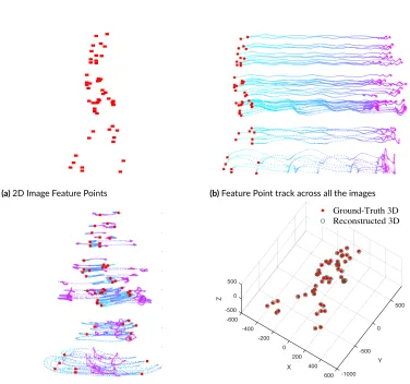
-2500 -2000 -1500 -1000 -500 0 500 1000 1500 -200

0 200 400 600 800 1000 1200 1400 1600 1800

(a)2D Image Feature Points (b)Feature Point track across all the images

(c)Mean centralized 2D features tracks

500 -500

-600

0 -400

Y

-200

X

0

-500 200

400

-1000 600 0

Z

500

Ground-Truth 3D Reconstructed 3D

[image:17.612.116.492.139.491.2]

(d)3D reconstruc on of the non-rigidly moving object Figure 1.3:A high-level illustra on of basic pipeline for 3D reconstruc on of a non-rigidly deforming object using fac-toriza on approach. (a) The 2D image feature for the ﬁrst image. (b) Feature tracks or trajectories of the 2D points across all the frames. (c) Mean centraliza on of the feature track to remove transla on component. (d) 3D reconstruc-on of the nreconstruc-on-rigidly moving object points. The above dataset is taken from walking sequence introduced by Torresani

(18)

and practically, that without any extra knowledge about the non-rigid object (other than low-rank) it’s possible to reconstruct the shape without any inherent basis-ambiguity. However, its performance on the benchmark dataset [6,168,93] is arguable. Therefore, the main con-cern is, with the recent theoretical surge in the understanding of NRSfM both theoretically and practically [44], Is SFM for any general non-rigidly moving object/scene is solved? At the time of writing this thesis, the answer remains ‘NO’!. Some of the reasons for this disap-pointing answer are listed in the following limitations.

Limitations

Even though few successful algorithms in NRSFM can provide satisfactory results, its still an unsolved problem for any general dynamic scene. The reasons are as follows:

• Most of the successful research in NRSFM assumes orthographic projection which limits its application to widely used perspective camera model.

• NRSfM methods assumes single non-rigid object is present in the scene for entire im-age sequence. In general, scene is composed of multiple moving objects.

• To realize per-pixel (dense) deformation of a shape, usually 3D templates are employed, which again is a non-practical and non-scalable approach to solve dense NRSfM. • One of the most important limitation of the NRSfM in general is the validity of the

correct representation of the deformation model. More precisely, which type of de-formation model can explain the non-rigidity of the object in the scene, for example low-rank, isometric deformation model, piece-wise rigid model etc. To me, its an open-problem.

Due to the above limitations, NRSfM algorithms are not widely applicable for practical pur-poses. In this thesis, we develop algorithms which enables new insight to solve NRSfM and provides some practical approaches to solve real world NRSfM problems. This thesis is also about realizing rigid 3D reconstruction problem as a small subset of problem available in this vastworld of non-rigidity.

(19)

model assumption. We slowly lift the insight of the readers and motivate them to think of any general dynamic scene as a global as rigid as possible scene, if observed closely within subsequent time frame (assuming this time is small enough), hence a NRSfM problem. To endorse our intuition we outline two methods to solve dense 3D reconstruction of a general dynamic scene. Finally, we provide the chapter-wise progression of the thesis from sparse to dense 3D reconstruction.

1.4 Prior-Free NRSFM Factorization: Modifications and Improvement Bregleret al.[21] matrix factorization approach proposed in the year of 2000 is one of the most widely used framework to solve NRSfM problem. After that, more than a decade of profound attempts to extend this framework were unable to provide a practical algorithm to solve this problem. Finally, it was in the year 2012 that Daiet al.provided a new insight to solve NRSfM which is popularly known as “prior-free” approach. The theory and algo-rithm proposed by Daiet al.[42] in a way changed the course of current research in NRSfM. However, overtime it was observed that their method fails to provide acceptable 3D recon-struction results on available dataset. As a result the prevailing view about this work is that it provides arguable results and hence, methods using compact data representation lashes on its performance [199]. So, the question we ask is Daiet al.seems theoretically correct but suffers practically “Why”?.

This thesis firstly provides the possible reasons for its practical failure. Our work gives an in-depth understanding of “prior-free” method and how some powerful elementary mea-sures and modifications can significantly improve its performance. We argue that byproperly utilizing the well-established assumption about a non-rigidly deforming shapei.e., it deforms smoothly over frames and it spans a low-rank space, the simple prior-free method can provide results which is comparable to the best available algorithms —at the time of writing this the-sis. Similar to prior-free method the only assumption we make is “low-rank” shape, and we show that a better solution to motion which satisfies smooth motion assumption is already present within the estimated “Gram matrix”, and explicit regularization on motion is not es-sentially required. Secondly, we propose how to better utilize the low-rank assumption. The improved performance is justified and empirically verified by extensive experiments on sev-eral benchmark datasets. Finally, this work also conjecture some theoretical problems which we think needs attention for further developments in factorization approach to NRSfM.

1.5 From single body to multi-body NRSFM.

(20)

consists of multiple objects undergoing non-rigid deformation. Therefore, we must look for an approach that solves multi-body NRSFM. One way to handle this it to solve 3D recon-struction task for each non-rigid object one at a time by pre-segmenting different objects in the scene. Nonetheless, its not a optimal way to solve the problem in which both the mo-tion and shape interacts. Under the assumpmo-tion that each non-rigid object spans a distinct globallinear subspace, this thesis present thefirstalgorithm to realize multi-body NRSfM [106]. To compactly represent complex multi-body non-rigid scenes, we propose to exploit the deformation in both spatial and temporal space, thus achieving a spatio-temporal rep-resentation. Specifically, we represent the 3D shape deformation in a union of subspaces in the temporal space and the 3D trajectories in the union of subspaces in the spatial space. Such spatio-temporal representation not only provides competitive 3D reconstruction but also gives reliable segmentation of multiple non-rigid objects present in the scene.

1.6 From Sparse NRSFM to Dense NRSFM

For many real-world applications, such as facial expressions, heart-surgeryetc, dense or per-pixel reconstruction of the object is very essential. NRSfM algorithms developed to recon-struct few sparse points of the non-rigid object fails to provide dense reconrecon-struction of the object and therefore, its unable to cater the subtle deformation in the object. The framework developed under the assumption ofgloballow-rank shape and the shape spansgloballinear subspace may not hold for dense deforming surface. The main reason for it is, any complex deforming surface can be composed of severallocallinear subspace structure. Therefore, the algorithm developed for sparse NRSfM fails to cater the inherentlocalstructure of the de-forming shape over space and time. This thesis lifts the intuition developed for union of subspaces in NRSfM problem and modifies it further to provide a scalable dense NRSfM al-gorithm. Our work utilizes Grassmannian representation to solve dense NRSfM which was previously studied only to represent set of images.

(21)

pro-pose two geometric algorithm that can help in achieving dense detailed 3D reconstruction of a dynamic scene under some mild assumption. Consider a general real-world dynamic scene, the change we observe in the scene between consecutive time frame is not arbitrary, rather it is regular. Hence, if we observe a local transformation closely, it changes rigidly, but the overall transformation that the scene undergoes is non-rigid. Therefore, to assume that the dynamic scene deforms as rigid as possible seems quite convincing and practically works well for most real-world dynamic scenes.

Importance

The topic covered in this thesis is of sheer importance to science and technology as it has tremendous application in medical, robotics, architecture, design, tourism, gaming, and many more. For instance, imagine a mobile robot which can capture the spatial layout of under-ground coal mine field, a precise medical surgery without any human supervision, automatic traffic or driving system, 3D models of your favorite monuments or building or actors, a truly immersed virtual reality experience for 3D game. All these application needs a robust dense 3D reconstruction of the involved scene. One can argue to use laser and depth sensing devices. However, such sensor is very costly with its own limitations and it is not portable enough to be embedded in smart portable devices with current technology. So, the argument here is; can we come up with some algorithm that uses the current imaging and computing resources to supply reliable geometry of a general dynamic scene.

1.8 Thesis Outline

After a brief introduction on structure from motion and brief overview of our thesis, we are ready provide progression of this thesis. At the beginning of each chapter in this thesis, we briefly discuss the motivation behind the concerned work. This discussion is followed by a comprehensive literature survey, where we review the relevant research area specific to topics covered therein. Our literature survey also tries to highlight the gray areas of the previous works.

(22)

experi-ments and results.

In Chapter (4) provides our work on dense non-rigid structure from motion which focuses on extending the idea of compact data representation using union of linear subspace to ob-tain per pixel 3D reconstruction of a deforming object.

An extension of the Chapter (4) is presented Chapter (5) where the motivation is to better uti-lize the Grassmannian representation developed in the previous chapter. The representation to group high dimensional data points inevitably introduce the drawbacks of categorizing samples on the high-dimensional Grassmann manifold. Therefore, to deal with such limita-tions, we propose to jointly exploits the benefit of high-dimensional Grassmann manifold to perform reconstruction, and its equivalent low-dimensional representation to infer suitable clusters. To achieve this, we project each Grassmannians onto a low-dimensional Grassmann manifold which preserves and respects the deformation of the structure w.r.t its neighbors. These Grassmann points in the lower-dimension then act as a representative for the selection of high-dimensional Grassmann samples to perform each local reconstruction.

In Chapter (6) we propose an efficient optimization framework to solve dense 3D recon-struction of complex dynamic scene using two perspective images. This work investigate on the rigidity of the scene using piecewise planar assumption. Under these assumptions, rel-ative scale of objects in the scene can be recovered faithfully. We describe the details of the formulations and its implementation followed by extensive experimental results. These ex-perimental results help conclude that dense detailed reconstruction using two perspective images is possible under some mild assumptions about the scene. In the following chapter (7), we took the assumption made in the Chapter (6) about a dynamic scene to next level. We proposed that if the depth for the reference frame is known a prior then we can estimate the dense depth map of a dynamic scene without using any 3D motion parameters.

1.9 State of the art

(23)

Algorithm Mean RMS Articulated Balloon Paper Stretch Tearing Multibody[106,104] 24.64mm 45.51mm 14.55mm 22.88mm 18.30mm 21.98mm

CSF2 [73] 26.09mm 35.51mm 19.01mm 33.95mm 23.22mm 18.77mm

RIKS [81] 26.75mm 42.11mm 18.45mm 32.18mm 22.88mm 18.12mm

KSTA [72] 26.86mm 35.63mm 24.88mm 31.96mm 24.25mm 17.59mm

MetricProj [136] 28.73mm 37.96mm 25.28mm 34.45mm 25.51mm 20.43mm

CSF [71] 30.83mm 36.84mm 30.43mm 32.17mm 28.87mm 25.82mm

PTA[8] 32.18mm 36.71mm 28.88mm 41.72mm 30.45mm 23.14mm

Bundle[46] 41.38mm 64.48mm 36.40mm 41.64mm 35.64mm 28.73mm

ScalableSurface[10] 41.84mm 58.12mm 31.71mm 45.45mm 38.88mm 35.03mm RigidTriangle [160] 43.83mm 65.71mm 34.38mm 43.57mm 40.54mm 34.94mm

SoftInext [180] 45.80mm 61.43mm 36.75mm 47.41mm 45.56mm 37.87mm

EM PPCA [167] 47.86mm 46.62mm 36.87mm 51.56mm 58.01mm 46.21mm

BALM [47] 48.79mm 75.09mm 35.84mm 53.13mm 40.31mm 39.58mm

Compressible [98] 59.98mm 72.77mm 52.53mm 62.44mm 57.45mm 54.71mm

SPFM [44] 63.81mm 89.40mm 45.65mm 64.19mm 64.04mm 55.79mm

MDH [32] 67.37mm 88.66mm 58.27mm 66.98mm 66.27mm 56.67mm

[image:23.612.105.560.226.496.2]

Concensus [115] 70.53mm 105.38mm 54.71mm 64.25mm 69.22mm 59.10mm

(24)

1.10 Preliminaries

Before we start to discuss on the problem of non-rigid structure from problem, we provide an overview on the basics of algebra and optimization concepts. The discussion on these topics by no means comprehensive, and is provided for the understanding and completeness of the thesis. In case the reader wants to get a very clear picture on most of the concepts used in this thesis, I strongly recommend to go through MIT Linear Algebra on-line course [157] and articles on the subspace clustering [181,182] and ADMM optimization [19].

(A) Trace of a Matrix: LetX∈Rn×n_{be a square matrix. The trace of the matrix}_X_is the sum of its main diagonal element. The trace of a matrix is also the sum of its eigen values.

Tr(X) = n

∑

i=1

Xii =x11+x22+x33+....+xnn = n

∑

i=1

λi(X) (1.1) where λi(X)refers to the eigen values of X.

Basic Properties

• Tr(X+Y) = Tr(X) +Tr(Y), AssumingX,Yare the matrix of same dimension • Tr(kX) =kTr(X), wherekis a constant.

• Tr(XY) =Tr(YX),X∈Rm×n,Y∈Rn×m • Tr(XTY) = Tr(XYT) =Tr(YTX) = Tr(YXT)

• Tr(XYZW) = Tr(YZWX) = Tr(ZWXY) = Tr(WXYZ)i.e., Trace is invariant under cyclic permutation

(B) Inner Product: Letx∈Rn,y∈Rnbe vectors of real numbers. The standard inner product onRn_{is given by}

<x,y>=xTy= n

∑

i=1

xiyi (1.2)

The standard inner product on real matrixX,Y∈Rm×nis given by

<X,Y>=Tr(XTY) = m

∑

i=1 n

∑

j=1

(25)

(C) Rank of a Matrix: The rank of a matrix is defined as the maximum number of lin-early independent columns/rows of the matrix. IfX∈Rm×n_then

0≤rank(X)≤min(m,n) (1.4)

The rank can be thought as the intrinsic dimension of the matrix. Any matrix of rankrcan be written as sum ofrrank-one matrixi.e.,

X= r

∑

i=1

λiuivTi (1.5)

Equivalently everym× nmatrix can be decomposed asX = UΣVT popularly known as singular value decomposition (SVD) whereU ∈Rm×r_{, Σ}_∈_Rr×r_and_V_∈_Rn×r_.

(D) Norms: The functionfusually denotes as∥.∥symbol: Rn _7→ _R

+is called norm if it

satisfies the following properties:

1. f is non-negativei.e., f(x)≥0, ∀x∈Rn 2. f is definitei.e., f(x) = 0 only ifx=0

3. f is homogeneousi.e., f(kx) = kf(x),∀x∈Rnandk ∈R

4. f must satisfy triangle inequalityi.e., f(x+y)≤f(x) +f(y),∀x,y∈Rn Exampl of vector norms

Letxbe a n-dimensional vector. The two very frequently usednormsarel1norm andl2 norm. Thel1andl2norm of a vector is given by

∥x∥1 =|x1|+|x2|+|x3|+...+|xn|= n

∑

i=1

|xi| (1.6)

∥x∥2 = (|x1|2+|x2|2+|x3|2+...+|xn|2)

1

2 =

n

∑

i=1

(|xi|2)12 (1.7)

More generallylpnorm forp≥1 is defined as

∥x∥p = (|x1|p+|x2|p +|x3|p+...+|xn|p)p1 ₌ n

∑

i=1

(26)

Asp→ ∞, thel∞norm orChebyshevnorm is defined as

lim

p→∞∥x∥p =max(|x1|+|x2|+|x3|+...+|xn|) (1.9) Example of matrix norms

LetX ∈ Rm,n_{be a matrix. Here, we will define some commonly used matrix norm in} literature.

• l1-norm of a matrix:

∥X∥1 = max 1≤j≤n

m

∑

i=1

|xij| (1.10)

• l2-norm or spectral or operator norm:

∥X∥2 =λmax(X) = (λmax(XTX)) 1

2 (1.11)

where,λmaxrefers to the largest singular value ofX.

• Frobenius Norm:

∥X∥F =√<X,X>=√Tr(XT_X_{) =}

v u u t∑r

i λ2

i (1.12)

where,λiis theithsingular value of the matrix andris the rank of the matrix. • Nuclear norm or Trace norm:

∥X∥∗ =

r

∑

i=1

λi(X) (1.13)

i.e., nuclear norm is the sum of singular values of a matrix. Hereris the rank of the matrix.

(E) Vector Spaces and Subspaces: Our brief discussion on this topic is inspired from Strang.G book [157] and Lecture 6 of MIT 18.06.

Letv,w∈Rnbe two vector in an-dimensional space. Thevector spacerequirements are: • If we add these two vector in the space, the answer stays in the same spacei.e.,v,w, and

(27)

a) Convex Set b) Non-Convex Set c) Non-Convex Set

Figure 1.4:Examples of convex and non-convex sets. (a) The square which includes its boundaries is convex (b) The pacman shaped set is non-convex, the line segment between the shown points in the set is not contained in the set. Similarly, set (c) is non-convex.

• If we multiply vectors with some scalars in the space, the answer remains in the same spacei.e.,v,kvare in the same space for some real numberk.

• All the linear combinationk1v+k2wstay in the same space. Herek1 andk2denotes any real numbers.

The vector space inside thisn-dimensional vector space is called thesubspaceofRn_{. The} subspace of a vector space is a set of vectors (including 0) that satisfies two requirements:If v,w are the vectors in the subspace and k any scalar, then

1. v+wis in the subspace. 2. kvis in the subspace.

3. All linear combination stay in the subspace.

(F) Convex Analysis: Here we will discuss some the basic definition that are important for the convex analysis an optimization problem. Our discussion is inspired from Boyd.S and Vandenberghe.L book on Convex Optimization [20].

Definition 1. A set C convex if the line segment between any two points in C li in C, i.e., if for any x1,x2 ∈C and any θ∈[0,1], we have

(28)

(a)Convex Func on (b)Non-Convex Func on Figure 1.5:Some examples of convex func on and non-convex func on

In other words, every point on the line segment connecting two points within the set lies in the set. Fig.(1.4) show some examples of convex and non-convex sets.

Definition 2. A function f:Rn _→ _R _{convex if domain of f} _{a convex set and if} _∀_x_,_y_∈ domain of f, and θ with0≤θ≤1, the following relation hold

f(θx+ (1−θ)y)≤θf(x) + (1−θ)f(y) (1.15) More specifically, the line segment joining(x,f(x))and(y,f(y))lies above the graph of functionf. The function is strictly convex if the above inequaltiy holds wheneverx̸=yand 0 <θ <1. Fig.(1.5) show some examples of convex and non-convex functions.

(G) Topological Manifold: A topologicaln-manifold (M) is atopological spacewhich islocally homeomorphicto an-ball (Bn_{), where}_n_{is a positive integer which is well-defined,} and it is the dimension of the manifold. Here, the space (M) is assumed to be Hausdorff and second countable. Fig.(1.6) shows an abstract example of a topological n-manifold.

Topological space: A topological space is a set endowed with the notion of open set and closed set.

Locally homeomorphic: Locally homeomorphic to an-ball means that every point in the space (M) contained in an open setOsuch that, there is a continuous one-to-one onto map f :O →Bn.

(29)

Figure 1.6:Visual intui on of a topological n-manifold. The do ed black-line along the boundaries of the circle denotes that the set is open.

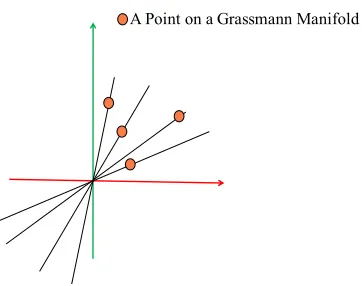
0<p ≤ d. Fig.(1.7) show each observation spans a one-dimensional subspace ofR2_, there-fore, its a point onG(1,2).

(H) Mathematical Optimization: A mathematical optimization problem has the form minimize

x f0(x)

subject to fi(x)≤bi,i=1,2, ....m

(1.16) Herexis the optimization variable of the problem, thef0is called the objective function or cost function. The functionsfi’s are the constraint functions (may be equality or inequality function) imposed on the optimization variable. The constant bi’s are the bounds for the constraint. The solution to the above cost function is considered optimal, if it has the smallest objective value among all the possible xthat satisfy the constraint. For more rigorous and detailed explanation on this, kindly refer to Boyd.S and Vandenberghe.L book on Convex Optimization [20].

(I) Low Rank Approximation Problem: The problem minimize

Y ∥X−Y∥ 2 F

subject to rank(Y)≤r where, X∈Rm×n

(1.17)

(30)

[image:30.612.219.400.93.236.2]

A Point on a Grassmann Manifold

Figure 1.7:Circled point represent a 1-dimensional subspace ofR2which is a point on Grassmann manifoldG(1,2).

replacing the remaining singular values by zeros. The result is referred to as the matrix ap-proximation lemma or Eckart–Young–Mirsky theorem [49]. More precisely,

(31)

2

Revisiting simple prior free approach to

NRSFM factorization

A simple prior free factorization algorithm[44] is quite often cited work in the field of Non-Rigid Structure from Motion (NRSfM). The benefit of this work lies in its simplicity of im-plementation, strong theoretical justification to the motion and structure estimation, and its invincible originality. Despite this, the prevailing view is, that it performs exceedingly inferior to other methods on several benchmark datasets[93,7]. However, our subtle investigation provides some empirical statistics which made us think against such views. The statistical re-sults we obtained supersedes Daiet. al.[44] originally reported results on the benchmark datasets by a significant margin under some elementary changes in their core algorithmic idea[44]. Now, these results not only exposes some unrevealed areas for research in NRSfM but also give rise to new mathematical challenges for NRSfM researchers. In this chapter, we will explore some of the hidden intricacies missed by Daiet. al. work[44] and how some elementary measures and modifications can significantly enhance its performance, as high as 18% on the benchmark dataset. The improved performance is justified and empirically veri-fied by extensive experiments on several datasets. We believe this chapter has both practical and theoretical importance for the development of better NRSfM algorithms. Practically, it can also help improve the recently reported state-of-the-art [104,93] and other similar works in this field which are inspired by Daiet al.work[44].

2.2 Introduction

Notation: For consistency and ease of understanding to the readers, the notation we used in th paper similar to Dai et al. work [44] unless otherwise stated. We assume that the reader

familiar with Dai et. al. work [44].

A simple prior-free method for computing non-rigid structure from motion (NRSfM) in-troduced by Daiet al.is now considered as a classical work in NRSfM [44]. In their work, the camera motion is estimated by imposing the null space constraint and the rank-3 positive semi-definite matrix cone constraint on the Gram matrix (Qk). Further, nuclear norm mini-mization of the reshuffled shape matrix (S♯_{) was introduced to proffer stronger rank bound}

(33)

(a)Paper Sequence

Ground-Truth Ours

(b)Paper 3D Reconstruc on

(c)Tearing Sequence

Ground-Truth Ours

(d)Tearing 3D Reconstruc on

Figure 2.1:The method recovers 3D dimensional structure of the deforming object over mul ple frames. Our elemen-tary but powerful changes provides a substan al improvement in the reconstruc on accuracy than the previous results reported for “prior-free” approach. The example images are taken from the recently released NRSfM Challenge Dataset [93]. Our reconstruc on results are nearly as good as the best performing algorithm without using very complex and involved mathema cal op miza on [104].

it not only challenged the myth of the inherent basis ambiguity in NRSfM [190] but also supplied a practical “prior-free” algorithm to solve NRSfM.

The elementary idea of Daiet al.[44] work conveniently encapsulates all the basic intu-itions which are required to solve a general NRSfM problem. One may immediately argue on its performance when the deforming shape is composed of a union of low-rank subspace [104,199]. However, in this chapter, we restrict our discussion to the classical representation of a NRSfM problem [22], without paying much attention to, how clustering benefits 3D re-construction of the non-rigid object and other such notions of compact data representation. The reason for this choice is that the improvement in the performance of a classical baseline will automatically benefit the methods built on top of it [104,199].

(34)

(S♯_{) is a far better choice than its global trace norm minimization. Lastly, due to our extensive}

analysis, we are able to posit some unsolved issues in NRSfM under “prior-free” idea which needs attention for further progress in this field.

It is not claimed that we achieve state-of-the-art results on the benchmark datasets us-ing our new approach. However, we empirically show that we can get very close to the best performing approaches and the difference is not very great, without the employment of com-plex and involved mathematical optimization [104,113]. In this chapter, we also argue that the inferior performance of “prior-free” method may not be due the proposed algorithmic idea but because they overlooked some of the mathematical construction in their own for-mulation, and missed on properly utilizing the well-known assumptions about non-rigidly moving objecti.e., smooth deformation[142] andlow-rank shape[44]. Hence, the conclu-sion, understanding and use of simple “prior-free” algorithm to NRSfM is not complete and precise. This chapter try to amend and nullify the prevailing perception about the “prior-free” approach, and how it can be used to its maximum potential. We feel that our work touches some critical points which are essential to establish a theoretical closure to some of the elementary problems within the factorization approach to NRSfM.

Contribution: Firstly, this work postulates some rectification to the usage of “Intersec-tion Method” [44] to compute camera motion. With the suitable example, we establish that the generalization made on the rotation matrix estimation by Daiet al.work [44] isnot con-vincing and therefore, the knowledge about the strength of “Intersection theorem” is not completely exploited. Secondly, we provide an analytic solution to estimate suitable rota-tion using Intersecrota-tion theorem and conjecture some challenges associated with it. Lastly, we propose a weighted nuclear norm minimization problem to estimate non-rigid 3D shape. Our approach shows a substantial improvement in the 3D reconstruction accuracy (as high as 17.6%). We also observed improvement in the performance of the algorithm in the presence of noisy data §2.5 and missing data §2.5 (with a minor adjustment).

In this work, our attempt is to make the baseline method*_{more accurate, both in terms of}

understanding and performance, subject to the mathematical simplicity. To achieve this, we attempt to avoid the usage of complex mathematical notions such as union of independent subspace, dependent subspace representation [199,104,112], procrustean normal distribu-tion [113], kernelization [72]etc. Hence, it is simple to understand the theoretical and prac-tical justification of our method. We show that by applying simple but powerful logical and mathematical modifications to prior free idea [44], we can get close to or even perform bet-ter at times than the best algorithms on the benchmark datasets. Additionally, our approach *_{By baseline, we mean the methods that solve NRSfM using its classical representation}_W₌_RS_{that have}

(35)

shall help improve the other state-of-the-art methods built on top of the targeted baseline [44].

2.3 Classical Representation

Tomasi and Kanade factorization method to structure-from-motion under orthographic cam-era projection appropriately summarizes the behavior of the 3D points over frames [164]. The relation between 3D shape, motion and its projection over frames was defined as

W=RS (2.1)

where,W∈R2F×P_{is the measurement matrix formed by stacking all the image coordinates} (x = [u,v]T) for ‘P’ points along ‘F’ rowsi.e., total number of frames.R = blockdiagonal

(R1,R2, ..,RF) ∈ R2F×3Fdenotes the orthographic camera rotation matrix with eachRi ∈

R2×3_{as per frame rotation.} _S _∈ _R3F×P_{represent the shape matrix with each row triplet as a} 3D shape. This representation was later extended by Bregleret al.[22] to recover non-rigid 3D shapes. More concretely,

W=



x11. . .. . .x1P

xF1. . .xFP

 =

 R..1S1

RFSF

 =



 c11R1. . .. . .c1KR1

cF1RF. . .cFKRF

 

 B..1

BK

 

⇒W=R(C⊗I3)B=ΠB

(2.2)

The matrix ‘B’ and ‘C’ are composed of shape bases and shape coefficients respectively, with ‘K’ as the number of shape bases. ‘⊗’ denotes the kronecker product and ‘I3’ is a 3×3 identity matrix. It is evident from the above formulation that the rank ofW≤3Kand also rank(S)≤ 3K. However,Sis not a general rank 3Kmatrix but own a special structure due toC⊗I3factor [44].

2.3.1 Null Space Representation to Orthonormality Constraint

An initial step in the factorization approach to NRSfM is to perform a rank 3K decompo-sition of the measurement matrixWvia singular value decomposition (svd)i.e.W = ˆΠB.ˆ This is then followed by the estimation of Euclidean corrective matrix ‘G’ to solve rotation and 3D structure. The main reason for such a procedure is due to the fact that the singular value decomposition of ‘W’ matrix is not unique as any non-singular matrixG∈ R3K×3K_in between the two matricesΠ andˆ Bˆcan form a valid factorization. Mathematically,

(36)

Now, once we are able to solveGcorrectly, then rotation and shape can be estimated using the above relations [22]. To solveG, orthonormality constraints are imposedi.e.RiRTi =I2. Representing theith_{double row of}_{Π as}ˆ _Πˆ

2i−1:2i ∈R2×3KandGk ∈R3K×3as thekthcolumn triplet ofG, then using Eq:(2.2) and Eq:(2.3) we can write

ˆ

Π2i−1:2iGk=cikRi,∀i={1,2, ..,F},k={1,2, ..,K} (2.4) Multiplying both sides byRT

i from right side gives ˆ

Π2i−1:2iGkGTkΠˆ T

2i−1:2i=c2ikI2

This leads to two linear equation constraint ˆ

Π2i−1QkΠˆ T

2i−1 = ˆΠ2iQkΠˆ T 2i ˆ

Π2i−1QkΠˆ T 2i =0

(2.5)

where,Qk ∈ R3K×3K = GkGTk. Using the algebraic relation vec(AXBT)=(B⊗A)vec(X), Daiet al.transformed these constraints (Eq:2.5) to a null space representation as follows:

[_ˆ

Π2i−1⊗Πˆ2i−1−Πˆ2i⊗Πˆ2i ˆ

Π2i−1⊗Πˆ2i

]

vec(Qk) =Avec(Qk) =0 (2.6) Using the above form and previous work in NRSfM [190], Daiet al.proposed the in-tersection theoremand supplied a SDP solution to estimate theQkmatrix and the Euclidean corrective matrixGkusingsvd().

Theorem 2.3.1. Intersection Theorem: Under non-generate and noise-free conditions, any cor-rect solution of Qk must lie in the intersection of the(2K2−K)dimensional null-space of A and a rank 3 positive semi-deﬁnite matrix cone i.e.Qkmust belong to

{Avec(Qk)} ∩ {Qk ⪰0} ∩ {rank(Qk) =3} (2.7)

2.3.2 Daiet al.solution to rotation

They proposed that once theQkis solved, rather than solving for full Euclidean corrective matrixG ∈ R3K×3K_{, use}_svd()_{to extract rank 3}_G

k. The solvedGk ∈ R3K×3 can then be use to findR(Eq:2.4) up to sign (cik). The method quote “we adopt a simpler approach

(37)

Gϵ ℝ3K×3K

G1 G) G3 GK

1: 3 4: 6 7: 9 3K − 2: 3K

[image:37.612.217.408.95.205.2]

Considered by Dai et.al.

Figure 2.2:(a) The column triplet (1:3) of euclidean correc ve matrix (Gk) used by Daiet al.work [44] shown in red shade. It is stated with the no on that there is no loss of generality to chooseG1. However, choosing

other column triplet may result in be er rota on and shape es mate as shown in Figure 2.4a and 2.4b

(a) When each column triplet{Gi}K

i=1qualifies for a suitable correction matrix, then why G1 has a high preference? Are we loosing useful information by such unwarranted preference? Whether such solution to rotation caters the assumption of smooth de-formation?

(b) Will each{Gi}Ki=1provide the same solution to the rotation matrix?

Daiet al.overlooked all these intrinsic issues with their approach to obtain rotation.

2.3.3 Plausible Rectification

Our experiment show that Daiet al.[44] solution to rotation estimation actually aborted the useful information present in theG ∈ R3K×3K_{. Each of the ‘K’ column triplets in}_G_(i.e.G

k) gives a possible rotation matrix which is different from each other (see Fig:(2.3)). Our em-pirical evaluations on several datasets show that the first column triplet isnotalways the best choice to estimate rotation. Hence, the details provided by Daiet al.work [44] isincomplete and there is aloss of generalitywith such procedure to estimate rotation under the well-known assumption of smooth deformation [142]. Fig:(2.4a) and Fig:(2.4b) provides few statistical results with comparison for both rotation and shape error estimate respectively. For clarity, we also provide the column triplet index that gives the better results for the corresponding data sequence and therefore, provides few counter-examples to such generalization.

(38)

provide better rotation and structure estimate (c) Upper bound on the value of ‘K’ which can guarantee a smooth solution. The problem seems hard keeping in view that the prior rank(K)in NRSfM factorization methods is an assumed approximation and it changes for different datasets to achieve better results.

2.3.4 A solution to motion

In this work, we use an analytical observation based on the smoothness and regularity† of the camera trajectory to filterGkto infer better rotation matrix. Letψ(.)be a function that takesGkas input and givesRas output using Intersection Theorem. We estimate different R ∈ R2F×3F for all the column tripletsi.e.{Gk}K_k=1, then computed the smoothness of the camera motion ‘δf’ for eachGkas:

Suppose,R=ψ(Gk), via Intersection method, then, δf =∥Rf−Rf+1∥2_F ∀f=1,2, ...,F−1.[84]Sec.4.

(2.8)

By examining the smoothness of the camera motion for eachGk, we select the suitable rotation matrix for structure estimation (see Fig. 2.3). Our strategy to select smooth camera motion over frames based on Eq:(2.8) consistently supplied us with better performance than the previously proposed approach. We acknowledge that this is not a profound way to in-fer the best rotation, however, it does provide a possibility to deduce better rotation using “prior-free” approach which respects the well-known assumption of smooth deformation in NRSfM. Further, it helps endorse our claim on the generalization of rotation estimate by [44]. You may use variable ‘δf’ Eq:(2.8) as a smoothness term in the final optimization (Eq:(2.11)) to further improve rotation, however, to show the competence within the “prior-free” framework [44], we stick to the classical way.

2.4 Structure Estimation

Once the rotation is estimated based on the smoothness of the camera motion, the next step is to solve for 3D structure. The block matrix method (BMM) by Daiet al.[44] proposed the following optimization problem to estimate the non-rigid low-rank shape.

minimize

S♯ ∥S

♯_∥

∗

subject to:

W=RS,S♯ =g(S)

(2.9)

(39)

0 50 100 150 200 250 300 350 400 0.115 0.12 0.125 0.13 0.135 De lt a

Consecutive Frames

(a)R←G1

De

lt

a

Consecutive Frames 0 50 100 150 200 250 300 350 400 0.11

0.12 0.13 0.14

(b)R←G2

De

lt

a

Consecutive Frames

0 50 100 150 200 250 300 350 400 0

0.05 0.1 0.15 0.2

(c)R←G3

De

lt

a

Consecutive Frames 0 50 100 150 200 250 300 350 400 0.115

0.12 0.125 0.13 0.135

(d)R←G4

De

lt

a

Consecutive Frames

0 50 100 150 200 250 300 350 400 0

0.05 0.1 0.15 0.2

(e)R←G5

De

lt

a

Consecutive Frames

0 50 100 150 200 250 300 350 400 0

0.05 0.1 0.15 0.2

(f)R←G6

De

lt

a

Consecutive Frames

0 50 100 150 200 250 300 350 400 0.115

0.12 0.125 0.13 0.135

(g)R←G7

De

lt

a

Consecutive Frames

0 50 100 150 200 250 300 350 400 0.11 0.115 0.12 0.125 0.13 0.135

(h)R←G8

De

lt

a

Consecutive Frames 0 50 100 150 200 250 300 350 400 0

0.1 0.2 0.3

(i)R←G9

0 50 100 150 200 250 300 350 400 0 1 2 3 4 De lt a

Consecutive Frames

(j)R←G10

De

lt

a

Consecutive Frames 0 50 100 150 200 250 300 350 400 0

0.5 1 1.5 2

(k)R←G11

De

lt

a

Consecutive Frames

0 50 100150 200 250 300 350400 0

0.5 1 1.5 2

(l)R←G12

Figure 2.3:The rota on samples onSO(3)using{Gk}12k=1forPick-up sequence. Below eachSO(3)manifold

is the graph showing the per frame change in the camera mo on using Eq:(2.8) ‘δf’. A simple observa on

establishes that all rota on matrix (R) are not the same. ‘δf’ graph analysis on this dataset show that the rota on es mate provided byG7,G8,G9has a smoother camera mo on than otherGk’s, withG9being the

(40)

(a)Mo on Improvement (b)Shape Improvement

Figure 2.4:Few counter examples on benchmark dataset [8]. (a) Rota on error in comparison to BMM [44] on synthe c data. (b) 3D reconstruc on error using global trace norm minimiza on of shape matrix as used in BMM with rota on matrix es mate using other column triplet in comparison toG(1:3). The column triplets of (G) for which the method perform be er on Pickup and Stretch sequence are (19:21), and (19:21)

respec-vely. Note that we used the same rank prior value ‘_K’ used in Dai_{et al.}work [44].

where,S♯ _∈ _RF×3P _{is a rearranged shape matrix with each row corresponds to the shape} for that frame. The trace norm minimization on ‘S♯_{’ is enforced instead of ‘S’ to provide a}

stronger rank bound on the shape matrix [44]. The second term in Eq:(2.9) enforces the re-projection error constraint. The functiong(.)mapsS ∈R3F×P_to_S♯ _∈_RF×3P_.

2.4.1 Daiet al.solution to shape

Following the work of Maet al.[123] on rank minimization problems, Daiet al.[44] proposed a solution to the optimization in Eq:(2.9). The method enforces low-rank constraint on ‘S♯_’

matrix and provide the solution by solving Eq:(2.9) via ADMM[19] using matrix shrinkage operatorS[λ](X)=Udiag(s[λ](σ))VT_{, where}_s_[_λ_](_σ₎₌_¯_σ_with_σ_¯

i=

{

σi −λifσi −λ > 0 and ‘0’ otherwise}.

2.4.2 Plausible Rectification

(41)

Conse-quently, nuclear norm minimization of the shape matrix struggles to appropriately conserve the useful component of the non-rigidly deforming shape.

Truncated nuclear norm regularization can be a choice to handle such issues, however, it depends on the binary decision, hence not versatile in nature [197]. To really cater the behavior of the deformations based on its low-rank nature, we propose to use weighted nu-clear norm minimization approach to solve for non-rigid structure [156,79]. In contrast to the previous notation to the nuclear norm of the shape matrixi.e.∥S♯∥

∗, we introduce a new

notation for its weighted nuclear norm ∥S♯∥Θ,∗ =

K

∑

j=1

Θjσj(S♯) (2.10)

whereσj(.)denotes thejthsingular value ofS♯. We assume that the weights Θj’s are non-negative scalari.e.Θj ≥0 . Using this representation, we redefine the optimization proposed in the Eq:(2.9) as follows:

minimize

S♯_,_S μ∥S

♯_∥Θ ,∗+

1

2∥W−RS∥ 2 F

subject to:S♯ =g(S)

(2.11)

The motivation for such formulation is quite clear, however, the proposed optimization (Eq:2.11) is generally non-convex, and is more difficult to solve than the nuclear norm mini-mization. Fortunately, recent results [196,122,79] in compressed sensing have shown that we can achieve a global optimal solution to Eq:(2.11) in the case when 0≤Θ1 ≤Θ2 ≤....≤Θ §2.4.3

2.4.3 A solution to shape

This section provides the mathematical derivation to the optimization proposed in Eq:(2.11). Our solution use the following theorems and proofs as stated and used in [196,79,27]. Theorem 2.4.1. For all Y ∈ Rm×n, denoted by Y = UΣVT, the SVD of it. The solution to minimizeX∥Y−X∥2

F +∥X∥Θ,∗, with non-negative weight vector Θ, its solutionX can beˆ

written Xˆ =UBVˆ T, whereBˆ the solution to the following optimization problem ˆ

B=argmin_B∥Σ−B∥2+∥B∥Θ,∗ (2.12)

Theorem 2.4.2. If the singular valu σ1 ≥....≥σKand the weights satisfy0≤Θ1 ≤Θ2 ≤

.... ≤ ΘK then the weighted nuclear norm minimization problem minimizeX∥Y−X∥2F + ∥X∥Θ,∗ h a globally optimal solution

ˆ

(42)

where Y = UΣVT the SVD of Y, andSΘ(Σ) the generalized soft-thresholding operator with weight vectorΘ

SΘ(Σ) = max(Σii−Θi,0) (2.14)

The readers are encouraged to refer to [196,79] work for detailed derivations to the lemma’s leading to the proof of the theorems. In conclusion, if the weights satisfies non-descending order, not necessarily with the same value, the weighted nuclear norm minimization problem is still convex and optimal solution can be obtained using a soft-thresholding operator with different weights [196,79].

Optimization: We propose our solution to the optimization problem defined in Eq:(2.11) using alternating direction method of multipliers [19] (ADMM), a simple, fast but power-ful algorithm used to solve many convex and non-convex problems in computer vision and mathematical optimization. The ADMM algorithm decomposes the original problem into several sub-problems, where each of them is solved separately by introducing Lagrange mul-tipliers and penalty parameters to estimate convergence. Using the method of mulmul-tipliers, the Augmented Lagrangian form for Eq:(2.11) is written as follows:

Lρ(S♯,S) = μ∥S♯∥Θ,∗+

1

2∥W−RS∥ 2 F+

ρ 2∥S

♯₋

g(S)∥2_F+

<Y,S♯−g(S)>

(2.15)

hereY∈RF×3P_{is a Lagrange multiplier and}_ρ_>_{0 is the penalty parameter. The solution to} each variable is obtained by solving the following subproblems over iterations (indexed with the variablei):

(S♯)i+1 =argmin

S♯ L

ρ((S♯)i,S) _(2.16)

(S)i+1 =argmin

S Lρ

(

S♯,(S)i) _(2.17)

The Lagrange multiplier and the penalty parameter are updated as follows: Y=Y+ρ(S♯−g(S))

ρ=minimum(ρ_max,λρ) (2.18)

ρ_maxrefers to the maximum value of ‘ρ’ andλis an empirical constant (λ > 1). The math-ematical derivations to each sub-problems are provided in the Appendix (A) for reference. The closed form solution to the Eq:(2.17) is obtained by taking the derivative of Eq:(2.15) w.r.t variable ‘S’ and equating it to zeroi.e.,

S=(ρI+R T_R ρ

)\((

g−1(S♯) + g

(43)

Note ‘\’ is a Matlab slangi.e.ifAx= Bimpliesx =A\B. Similarly, rewriting the Eq:(2.15) treatingS♯_{as variable.}

=argmin

S♯

μ∥S♯∥Θ,∗+

ρ 2∥S

♯₋

g(S)∥2_F+<Y,S♯−g(S)> _(2.20)

In contrast to the previous form, the solution to Eq:(2.20) is not straight forward. To obtain a closed form solution to this problem, lets define a soft-thresholding functionS[τ](σ) = sign(σ).max(|σ| −τ,0). Also, let[U,Σ,V]be the singular value decomposition of (g(S)− Y/ρ), then the optimal solution to Eq:(2.20) is given by:

S♯=US[Θμ

ρ ](Σ)V (2.21)

Here, Θ is the weight assigned to the different singular values in the non-descending order based on its significance to the deformation data. For detail discussion on the initialization of weights refer section §2.5 (2). Its important to note that the ADMM based solution to our optimization problem Eq:(2.15) gives us a satisfactory solution (near optimal) which may not be globally optimal.

2.5 Experiment and Discussion

To endorse our claim, we performed extensive experiments on real and synthetic benchmark datasets [7,93,169]. We compared the performance of our algorithm against different state-of-the-art methods on these datasets [73,113,104]. Additionally, we unveil the substantial percentage boost in the reconstruction accuracy as high as 18% in comparison to the previous results reported for “simple prior-free” approach. For real-world applications to NRSfM, noisy data and missing feature tracks over frames are crucial, therefore, we also performed experiments to tackle such issues. Before we provide details on the performance analysis, we discuss the variable initialization.

Initialization: Our algorithm has few parameters and variables to initialize. For all our experiments on different datasets, we initializeμ = 1, λ = 1.1, ρ_max = 1e10, ρ = 1e−4, Y = zeros(F,3P)and the ‘K’ values are kept same as Daiet al.method[44]. Practically, we considered the convergence of our optimization, if the gapmax_∥(S♯ ₋_g₍_S₎₎_∥

∞ < 1e−8 or

ρ>ρ_maxover iteration.

1. Structure initialization: Using the result of Liuet al.[118] on the uniqueness of mini-mizer for the rank minimization problem, we initialize the the 3D shape ‘S’ as ‘S’ =pinv(R)W andS♯ ₌_g₍_S₎_{. The pseudo-inverse solution to shape matrix provides a good enough}