S T A T I S T I C A L M O D E L S
F O R
M U L T I L O C U S S T R U C T U R E S
BY
C
hristopher
E
ric
A
ston
A thesis submitted to the Australian National University
for the degree of Doctor of Philosophy
in the
Department of Statistics Research School of Social Sciences
Except where otherwise stated, the work presented in this thesis is my own.
A c k n o w l e d g e m e n ts
My sincere thanks to my supervisor, Dr S.R. Wilson, for introducing me to the subject of data analysis in genetics and for the assistance and encouragement she gave me during my studies at the A.N.U.
I am indebted to Tony Brown, Sue Serjeantson, John Oakeshott and Gordon Smyth for many enlightening discussions. I would also like to thank the helpful
staff of the Computer Services Centre and in particular, Kathy Handel, Jeff Brindle and Geoff Barlow. To my
friends, for their support and generous offers of help, thank you. For an excellent typing job my thanks
S u m m a ry
In this thesis methods are considered for analysing relationships between genetic systems, usually loci, in an organisms genome. In particular, the genome of the individuals are typed at several sites.
Chapter 1 provides an introduction to and
motivation for the areas covered in this thesis. The remaining chapters are divided into two parts.
Part I, comprising chapters 2 and 3, deals with the analysis of multilocus data in population genetics, and in particular, plant genetics. Chapters 4, 5 and 6 form Part II which looks at the analysis of multilocus data in the context of medical studies.
Summary measures of pairwise nonrandom allelic association are studied in chapter 2. An alternate form of an existing summary measure is proposed. The sampling properties of both these measures, and of tests for detecting nonrandom allelic association based on these measures, are studied using computer simulations.
The application of log-linear model analysis to data on multiple sites is outlined in chapter 3.
iv.
large tables a modification of the usual test
procedures utilised in log-linear model analysis is
proposed. A stepwise procedure for detecting nonrandom allelic associations is described and applied to wild barley data.
Turning to more medically orientated problems chapter 4 considers genotypic data for diploid organisms in which the constituent gametes are not
identified. A composite link function is used to adapt
log-linear model analysis to these data. Application to artificial data sets is used to justify this
computationally more complex approach.
In chapter 5 attention is turned to linkage analysis of family data where individuals have been typed for
multiple markers/loci (usually referred to, in this context, as multipoint data). A multipoint linkage analysis is proposed and applied to artificial family data. Extensions of this multipoint linkage analysis and its role in general linkage analysis are discussed.
The thesis concludes with chapter 6. This chapter describes the implementation of the multipoint linkage analysis given in chapter 5.
Some of the results in chapter 5 have been
published in Aston and Wilson (1985) and Aston (in press). A modified version of chapter 4 is to be published
(Aston and Wilson: Log-linear model analysis of allelic
V.
C o n t e n t s
1. Introduction 1
P a r t I
2. Examination of a summary statistic for pairwise nonrandom allelic association
2.1 Introduction 5
2.2 Simulation results 9
2.3 Discussion 19
3. Detecting nonrandom allelic association utilising log-linear models
3.1 Introduction 21
3.2 The proposed stepwise procedure 25
3.3 Application of this stepwise procedure
to barley data 31
3.4 Empirical results for the test procedures
P a r t II
4. Detecting nonrandom allelic association in multilocus genotypic data.
4.1 Introduction 40
4.2 The composite link function approach 42 4.3 An approach assuming equiprobable phases 48
4.4 Application to some simulated data 49
4.5 Extensions to the composite link approach 60
5. Multilocus linkage analysis
5.1 Introduction 62
5.2 An algorithm for multilocus linkage analysis 64 5.3 Application to some artificial family data 74
5.4 Discussion 80
6. A multilocus linkage analysis program
6.1 Introduction 86
6.2 A database for family data 87
6.3 The implementation of the approach to
multilocus linkage analysis 102
6.4 Discussion 119
References 123
Appendix
A .1 Analysis of deviance tables (Part A) 128 A.2 Analysis of deviance tables (Part B) 133 A.3 Models utilised to obtain "Empirical results
for the test procedures". 136
1.
C H A P T E R 1
I N T R O D U C T I O N
This thesis presents a discussion of statistical methods of detecting nonrandom allelic association in multilocus data. These statistical methods are developed
for data arising from two different contexts, namely for multilocus gametic data in (plant) population genetics and multilocus genotypic data in medical genetics. This forms the basis for parts I and II of this thesis
respectively.
Gametic data is characterised by the researcher knowing the constituent gametes forming an individual's genotype, (also termed as knowing the phase of an
individual's genotype). Typically, gametic data are collected in population genetic studies of plants or invertebrates as these are amenable to techniques, such as progeny testing, which are used to distinguish the analogous forms of multiple heterozygotes. In
particular, for gametic data collected in studies of
cultivated plants, detecting nonrandom allelic association is of interest in, for example, crop improvement
2.
"presence of [nonrandom allelic association] can
adversely affect selection experiments/trials, a 'good'
allele may be associated with a poor gamete" (Wright, 1983). Thus, for example, selection of crops for high yield may result in low disease resistance.
Brown, Feldman and Nevo (1980) proposed a test for the presence of nonrandom allelic association based on a summary measure of heterozygosity. To do this they assumed, with reservations, that this summary measure is normally distributed. This assumption is examined by computer simulation in chapter 2 and the evidence suggests that this assumption is untenable. An alternative test based on a modified form of this summary statistic is proposed and the properties of this test examined by computer simulation. These summary measures entail a severe loss of information regarding the structure of any nonrandom allelic association detected.
3.
procedures used in log-linear model analysis are not appropriate and these have been replaced by Monte Carlo test procedures (as suggested in Aston and Wilson, 1984).
The properties of these test procedures are examined by computer simulation. This modified log-linear model analysis is applied to the data on wild barley (Hordeum
spontaneum) analysed by Brown et a l . (1980). These methods
assume gametic data are available. However, in many studies only genotypic data are available.
In genotypic data the constituent gametes of an
individual are indeterminant and so genotypic data can be regarded as being incomplete. Such is the usual form of data collected in medical genetic studies and it is in this context that genotypic data are considered here. Study of the genetics of the histocompatability system in humans where knowledge of associations between the loci making up the system may help improve techniques of tissue matching for organ transplants is an example. An adaptation of the methods suggested by Thompson and Baker (1981) for applying log-linear model analysis to genotypic data is described and discussed in chapter 4.
Often genotypic data may be available for individuals which are grouped in families. Here, linkage analysis
is used to detect nonrandom allelic association where association (termed 'linkage') is assumed to be due to the loci being on the same chromosome. Linkage analysis
198 5, (see Con n e a l l y and Rivas, 1980, and White et a l.,
for r e v i e w s ) . A lthough methods of detecting linkage
between pairs of loci are well developed, little has been
done on detecting linkage between multiple loci. An
a l g o r i t h m is given in chapter 5 for multi l o c u s linkage
analysis together with results of its a pplication to
artificial family data. The programs written to implement
5.
PART I
Mu lt i l o c u s Data in Populati on Genetics
CHAPTER 2
e x a m i n a t i o n o f a s u m m a r y s t a t i s t i c f o r p a i r w i s e n o n r a n d o m a l l e l i c a s s o c i a t i o n
2 .1
I n t r o d u c t i o n .
The first part of this thesis is concerned with the analysis of multilocus gametic data with particular emphasis on data for plants. Gametic data are easily obtained for many plant species of commercial interest because of their high homozygosity and ease of progeny testing. The
multilocus gametic data utilised throughout part I of this thesis are from a survey of twenty-six natural populations of wild barley (Hordeum spontaneum) in Israel. A description of these data is given in Brown, Feldman and Nevo (1980) .
6 .
linkage disequilibrium. This term is a misnomer for
two reasons. First, the observed nonrandom associations between alleles are not necessarily caused just by
linkage (the physical association of loci on the same chromosome) alone. The associations could be due to a combination of linkage, inbreeding, selection and so on. Second, several theoretical models for genetic systems have been developed which predict equilibrium points at
which there is stable disequilibrium. To avoid this
confusion the term nonrandom allelic association is adopted.
A common basis for measuring nonrandom allelic association between pairs of alleles is the statistic
defined as
3 ^
(2.1) ik _ ik i k
J £ $ c l P j PI
ik
where g .0 is the frequency of the gametes carrying the
J &
ith allele at the jth locus and the kth allele at the
p
£th locus; p . is the frequency of the ith allele J
at the jth locus. This measure can be generalised to higher order associations involving three or more loci
(see, for example, Brown, 1975). However, for multilocus gametic data the large numbers of such ^-statistics are difficult to interpret biologically.
7.
in a zygote formed by artificially combining two randomly chosen gametes. This variance (a2) can be written as
(2.2) 2 l l 1112p) p\
3 3 3 3 Jl>3 i k 3
+ i D \ k ) 2 ]
J Ä
where h
locus. Hence, the variance (g2) is cumulative over locus pairs, tending to increase with "more" pairwise association
(although, for some combinations of allele frequencies this is not the case) but is independent of higher order
associations. To calculate g2 the distribution of the number of heterozygous loci is obtained by comparing each gamete with every other gamete in a sample of n gametes (giving (^) comparisons). Let s 2 be the observed value of this variance (o2) then under the hypothesis (H ) of random association of alleles
i -
U
p))
i C
is the gene diversity at the jth
(2.3) E (s 2 IH is true) = ] h . (1 -h .)
° 3 3 3
and to order n
(2.4) Var (s2 |H is true) h . - l) h 2.
6 J o J
+ 12 y h 3.-6l h\ + 2 [ I h . (1 - h .) ] 2}/n
J J J
J6
J Jwhere the parametric values of the {h .} are replaced by their estimates.
8.
consisted of computing a one-sided confidence interval
for the variance ( o 2 ) assuming that the sampling
distribution of the variance statistic is2) could be
approximated by a normal distribution. Thus the hypothesis Hq is rejected on the available evidence at a nominal
5% level of significance if the observed value, s2 ,
exceeds the value L given by
(2.5) L =E(s2 |h is true) + 1.69 x Var(s2 |H is true) 2.
However, they do state that, "it is not clear whether the sampling distribution of [s2] is normal or whether another approximation would be appropriate".
An alternative test for pairwise nonrandom allelic association is proposed based on a suggestion by B. Manly
(Pers.Comm.). Here, the hypothesis (H^) , as given above, is rejected at a nominal 5% level of significance
if the test statistic X , given by
( [j] - 1 U 2
(2.6) X = --
---E(42 IHq is true)
exceeds the value of the 5% point of a chi-squared distribution with degrees of freedom v = [~\ - 1
([ ] = 'the integer part of') . Here, the values s2 and E(s2 |Hq is true) have been replaced by the values
4 2 and E (4 2 IH is true) calculated from the 1 o
distribution of heterozygous loci obtained from a single random sample of [— ] - 1 pairs of gametes from the
9. of the observed variance was introduced because of the
correlations between the (^) pairs of gametes used to
calculate s 2 . Computer simulation studies by the author and Lonie (1984) showed that these correlations caused the sampling distribution of the statistic X to
have a variance greater than 2v . However, this
sampling of [— ] gamete pairs does involve an extraneous sampling variation and some loss of information.
The properties of these tests and the distributional assumptions on which they are based are investigated by computer simulations in the following section. This chapter concludes with a discussion of these results and of these measures of pairwise nonrandom allelic association.
2 . 2 S i m u l a t i o n R e s u l t s .
The method of generating the data in the simulation study was as follows. Under the assumption that there are no nonrandom allelic associations, expected frequencies can be calculated for the multilocus gametes from given
sets of allele frequencies. Simulated data sets were then obtained as observations from multinomial distributions with the appropriate expected frequencies. These
observations were generated using the IMSL subroutine GGMTN (IMSL, 1982). It was decided to generate two
thousand data sets for each choice of allele frequencies.
The simulations are in two parts, A and B .
1 0.
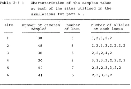
barley populations referred to in section 2.1 were used. Some of the characteristics of the samples taken at each
of these six sites are given in Table 2-1.
Table 2-1 : Characteristics of the samples taken at each of the sites utilised in the
simulations for part A .
site number of gametes sampled
number of loci
number of alleles at each locus
1 30 5 3,2,3,2,2
2 48 8 2,3,3,3,2,2,2,2
3 38 5 2,2,2,4,2
4 30 8 3,2,3,3,2,2,2,2
5 52 7 2,3,2,3,3,2,2
6 41 5 2,3,3,3,2
Part B consists of several artificial sets of allele frequencies in which the effects of characteristics of the generated artificial data on the properties of the measures and tests could be studied. The particular characteristics varied here were the following :
the size of the data set as determined by the number of loci (4,6,8) and the number of alleles at each locus
(2,3,4) ; the number of gametes sampled (25,100) ; the homogeneity of the allele frequencies at each locus
[image:17.557.85.509.181.469.2]1 1.
data and values for which the simulations were
computationally tractable.
The assumption of normality for the variance
statistic i s 2 ) was examined using the Shapiro-Wilk
test of normality (Shapiro and Wilk, 1965). In this
context, the Shapiro-Wilk test consisted of calculating
the test statistic W , given by
25 { I a
i = l 50-i+l y 50-i+l - y jy i } 2 (2.7)
50
I (2/v-
y )i = l ^
where ^ are orc^er statistics (in ascending
order) for a sample of fifty s 2 values ; y is the
2 5
mean of this sample ; ^ a 50-i + l - -1 are coef ficients
which are tabulated in Shapiro and Wilk (1965). The
hypothesis of normality of the sampling distribution of
the variance statistic (s2) is rejected at a 5%
level of significance if W < 0.947 . The numbers of
tests rejecting the hypothesis of normality for the
variance statistic i s 2 ) out of forty Shapiro-Wilk tests
applied to the generated data for each set of allele
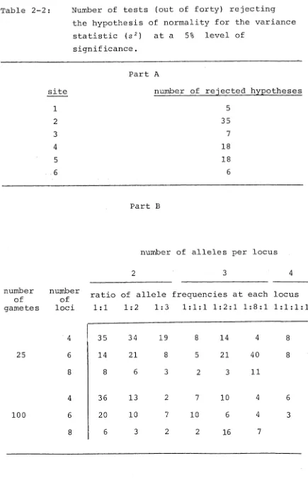
frequencies are given in table 2-2. The expected number
of tests rejecting the hypothesis, out of forty, is 2
if the sampling distribution of the variance statistic
(s2) is normal. The results in table 2-2 suggest that
the assumption of approximate normality is not appropriate
for the sampling distribution of the variance statistic
1 2.
Table 2-2: Number of tests (out of forty) rejecting
the hypothesis of normality for the variance
statistic (s2) at a 5% level of
significance.
site
1 2
3
4
5
6
Part A
number of rejected hypotheses
5
35
7
18
18
6
Part B
number of alleles per locus
2 3 4
number of gametes
number of loci
ratio
1:1
of allele
1:2 1:3
frequencies at each
1:1:1 1:2:1 1:8:1
locus
1:1:1
4 35 34 19 8 14 4 8
25 6 14 21 8 5 21 40 8
8 8 6 3 2 3 11
4 36 13 2 7 10 4 6
100 6 20 10 7 10 6 4 3
[image:19.557.75.510.75.773.2]1 3.
This contradicts the conclusion drawn by
Chak r a b o r t y (1984). Chak r a b o r t y concluded in favour of
n o r mality b a s e d on the observed values of the coeffic i e n t s
of skewness and kurtosis of the sampling distribution of
the variance statistic (s 2 ) (given here in table 2-3)
obtained from generated data sets for two diallelic loci.
Table 2-3: Values of skewness (y) and kurtosis (k)
of s 2 taken from table 1 of
C h a k raborty (1984).
p ! = 0 .25 P i = 0 .5
p 2 = 0.1 p 2=0.3 p 2=0.5 p a= 0.1 p 2=0.3 p 2=0.5
number of gamete s
100
1000
Y .197 .057 .012 .132 .028 .004
K -.843 -.838 -.289 -.828 -.648 -.035
Y . 062 . 056 . 031 .036 .012 .003
K -.783 -.548 -.219 -.129 -.125 .027
In figure 2-3, pi and p 2 are the probabilities
of the first allele at locus 1 and 2 respectively.
Skewness (y) = m 3 / m 2 /rn^ and kurtosis (k) = (m ^ / m l) - 3
were c omputed from the observed central moments of s 2
over ten thousand generated data sets for each
1 4. For the normal distribution the expected values for the skewness and kurtosis measures used by
Chakraborty are zero. Considering that each of the values in table 2-3 was obtained from ten thousand generated data sets, the values, especially for kurtosis (k) , appear to be significantly non-zero except when the allele
frequencies are approximately 0.5. (Estimates of standard errors would be necessary to substantiate this observation.)
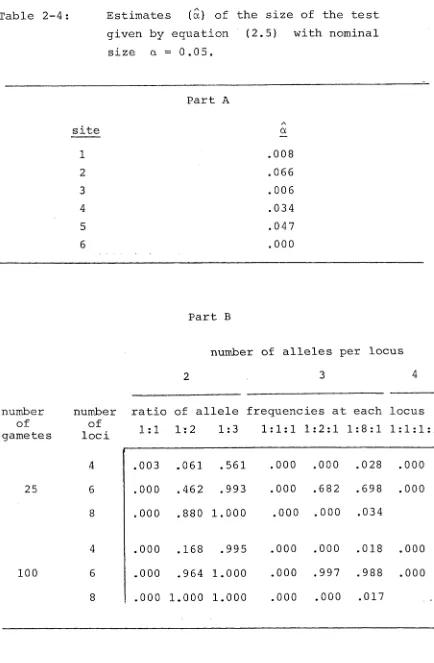
In table 2-4 are estimates (a) of the size of the test suggested by Brown et al. (1980) , and given by equation
(2.5) , which has nominal size a = 0.05 . Each estimate
A
(a) is calculated from tests applied to the two thousand data sets generated from each set of allele frequencies.
Table 2-4 shows that the estimated size of the test suggested by Brown et a l . (1980) is strongly dependent upon the characteristics of the data set. The estimated
size of the test is much smaller than the nominal size 0.05 when the allele frequencies are uniform at each locus (that is, in the ratios 1:1, 1:1:1 or 1:1:1:1). However, as these frequencies become less uniform at each locus and the number of alleles at each locus increases the estimated size becomes much larger than the nominal size 0.05.
The remaining results concern the alternative test
1 5.
Table 2-4: Estimates (a) of the size of the test given by equation (2.5) with nominal size a = 0.05.
Part A site
/\
a
1 .008
2 .066
3 .006
4 .034
5 .047
6 .000
Part B
number of alleles per locus
2 3 4
number of gametes
number of loc i
ratio 1:1
of allele frequencies at 1:2 1:3 1:1:1 1:2:1
each 1:8:1
locus 1:1:1
4 .003 .061 .561 .000 .000 .028 .000
25 6 .000 .462 .993 .000 .682 .698 .000
8 .000 .880 1.000 .000 .000 .034
4 .000 .168 .995 .000 .000 .018 .000
100 6 .000 .964 1.000 .000 .997 .988 .000
[image:22.557.76.510.84.747.2]16 .
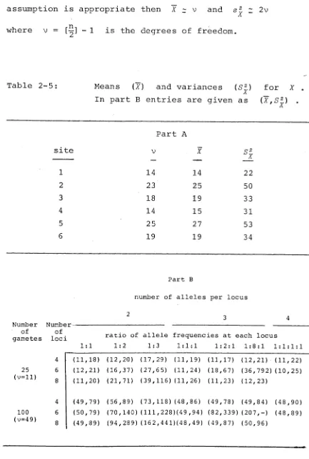
assumption is appropriate then X 2 v and s 2 z 2 v
X
where v = [^-] - 1 is the degrees of freedom.
Table 2-5: Means (X) and variances (S 2 ) for X . A
In part B entries are given as (~X,S2 ) . A
Part A
site V X q 2
b x
1 14 14 2 2
2 23 25 50
3 18 19 33
4 14 15 31
5 25 27 53
6 19 19 34
Part b
number of alleles per locus
Number Number
of of
gametes loci ratio of allele frequencies at each locus
1 : 1 1 : 2 1 :3 1:1 : 1 1:2:1 1:8:1 1 :1:1 : 1
4 (11,18) (12,20) (17, 29) (11,19) (11,17) (12,21) (11,22)
25 6 (12,21) (16,37) (27, 65) (11,24) (18,67) ( 3 6 , 7 9 2 ) ( 1 0 , 2 5 )
(v=ll)
8 (11,20) (21,71) (39, 116) (11,26) (11,23) (12,23)
4 (49,79) (56,89) (73, 118) (48,86) (49,78) (49,84) (48,90)
100 6 (50,79) (70,140) (111 , 2 28)(4 9,94) ( 8 2 , 3 3 9 ) ( 2 0 7 , - ) (48,89)
(v = 4 9)
[image:23.557.77.510.64.708.2]17.
' ' TThe evidence in table 2-5 suggests that the sampling dlistribution of X can be appropriately approximated ■ b:>y a chi-squared distribution when the allele frequencies • • aire uniform at each locus, although the sampling
dlistribution appears to be less dispersed (sj < 2v) A
tthan a chi-squared distribution. However, the
aappropriateness of the chi-squared distribution is lost aas the number of alleles at each locus increases and the aallele frequencies move away from uniformity.
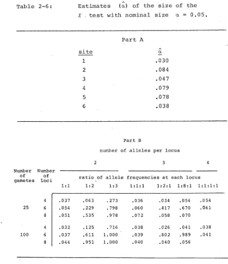
Estimates (a) of the size of this X test with mominal size a = 0.05 are given in table 2-6 . Each eestimate was calculated from tests applied to each of the ft wo thousand simulated data sets generated for each set cof allele frequencies.
In table 2-6, for uniform allele frequencies, the ^estimated size of the X test appears to be close to tthe nominal size of 0.05 . Nevertheless, as for ttable 2-4, the estimated size is much larger than the
mominal size 0.05 as the number of alleles at each locus ^increases and the allele frequencies move away from
lunif ormity.
A
Some estimates (II) of the power of the X test vwere obtained. These estimates suggested the X test
/\ /\
lhas poor (IT = 0.1) to moderate (IT = 0.5 to 0.7) jpower. No systematic study of the power of this
Table 2-6:
18
Estimates (a) of the size of the
X . test with nominal size a = 0.05.
Part A
site a/X
1 .030
2 .084
3 .047
4 .079
5 .078
6 .038
Part B
number of alleles per locus
Number of gametes
Numbe of loci
2 3 4
1 :1
ratio of allele 1:2 1:3
frequencies at each locus
1:1:1 1:2:1 1:8:1 1:1:1:1
4 .037 .063 . 273 .036 .034 .054 .054
25 6 .054 .229 . 798 .060 .417 .670 .061
8 .051 .535 .978 .072 .058 .070
4 .032 .125 .716 .038 .026 .041 .038
100 6 .037 .611 1.000 .039 .802 .989 .041
[image:25.557.52.505.79.604.2]1 9.
2 . 3 D i s c u s s i o n .
The evidence given in section 2.2 suggests that caution is required when using the test proposed by Brown et a l. (1980) for detecting pairwise nonrandom
allelic association. On the one hand, for uniform allele frequencies the test is conservative in the sense of
failing to reject a null hypothesis which might otherwise have been rejected by an exact size a = 0.05 test.
On the other, the reverse occurs when allele frequencies are not uniform and many loci are studied. What effect these results have on the interpretation of the
conclusions in published studies utilising this test is uncertain.
An alternative test for detecting pairwise nonrandom allelic association utilising the statistic X given by equation (2.6) appears, for uniform allele frequencies, to have size a ~ 0.05 and a more appropriate
distributional assumption as its base. Nevertheless, caution is required with its use because of the low power of this test and its poor performance when allele
frequencies are not uniform.
However, using any test based on the summary statistic
s 2 (or 42) incurs a severe loss of information concerning the structure of the nonrandom allelic
associations. On the other hand for multilocus data the more usual method of calculating ^-statistics leads to
2 0.
simultaneously. The analysis of nonrandom allelic association described in the next chapter offers a
2 1.
C H A P T E R 3
D E T E C T I N G N O N R A N D O M A L L E L I C A S S O C I A T I O N
U T I L I S I N G L O G - L I N E A R M O D E L S
3 . 1 I n t r o d u c t i o n .
In this chapter an approach using log-linear models
is p r o p o s e d for detecting n o n r a n d o m allelic association
between loci in multilocus gametic data.
This approach formulates multilocus gametic data as
a cont i n g e n c y table by represe n t i n g each locus by a
categorical variable (or factor) and each allele by a
level of the c o r r esponding categorical variable. Such
tables c o u l d be analysed by classical log-linear model
analysis as described by Bishop, Feinberg and Holland (1975)
or M c C u l l a g h and Neider (1983). In this classical a p proach
the N mu l t i l o c u s gamete frequencies Y^ (corresponding
to the N cells of the contingency table) are assumed
to be independently Poisson d istributed with E(Y^.) = y^ .
The dependence of the mu l t i l o c u s gamete frequencies Y^
on the c ategorical variables (the loci) is given by
2 2.
where x . is a p x 1 vector of explanatory variables
~ is
(dummy variables for levels of factors)and 3 is a
T
P* 1 vector of parameters 3 = (3j - - • '3^) • The problem of modelling is then to find an appropriate
parsimonious model, with model matrix X of order N x p,
which satisfies some criteria for goodness-of-fit.
A commonly used measure of goodness-of-fit of a model is the deviance, Z?(z/;y) , given by
N
(3.2) 2 {E - {ij ^ - y £ }
i— 1
where y are the observed multilocus gamete frequencies and y are the fitted values derived from a model involving a particular choice of X . The test procedures usually used to assess the goodness-of-fit of a model assume that the deviance statistic is asymptotically distributed like a chi-squared. An alternative is to test differences between the deviances for two models from a seauence of nested models (that is, the parameter space of one model represents a subspace of the parameter space of the other). This deviance difference provides a measure of
improvement-of-fit due to those parameters by which the two models differ and is also usually assumed to be
asymptotically distributed like a chi-squared. However, contingency tables formed from multilocus gametic data are typically large and very sparse. (For example, for
2 3.
their cells containing zero frequencies*) As a consequence, these chi-squared assumptions are
inappropriate. In the approach described here these usual test procedures are replaced by Monte Carlo test procedures.
A Monte Carlo test of the goodness-of-fit of a
model M with model matrix X consists of the following. A 'reference set' is formed as a group of data sets generated in accordance with the hypothesis (H ) that
M is the true model for the observed data. Each of these
X-l generated data sets are simulated as observations from a multinomial distribution with expected frequencies given by the fitted values obtained for the model M
from equation (3.1) . Here the data simulation process utilised the IMSL subroutine GGMTN (IMSL, 1982).
The model M is then fitted to each of the K-l generated data sets and a group of K-1 deviance statistics
calculated using equation (3.2) . The hypothesis (H^) is rejected at a level of significance a if the
observed deviance statistic is the #ath largest or larger deviance statistic relative to the deviance statistics derived from the 'reference set'. (X and are
positive integers.) A Monte Carlo test of the improvement- of-fit, based on the deviance difference statistic, follows the same procedure mutatis mutandis. This procedure is exact in the sense that the type I error is precisely a for all choices of K (Hope 1968). Marriott (1979, and references therein) suggests K should be chosen so
24 .
to generate reference sets for large, sparse contingency
tables for several tests of hypotheses led to the choice
of the values K — 20 , Ka = 1 . Empirical estimates of size and power for this Monte Carlo test (with K = 20,
= 1) are given in section 3.4. A stepwise procedure for the detection of nonrandom allelic association using a log-linear model analysis incorporating the above test procedure is described in section 3.2. The results
obtained by applying this procedure to the wild barley data referred to in chapter 2 are given in section 3.3.
As an aside, it is noted that, in tests of
improvement-of-fit, (nuisance) parameters of little or no relevance to the test may be involved. For example, parameters for the main effects (re allele frequencies) are of little or no relevance to tests of the
improvement-of-fit due to an association. Classical log-linear model analysis eliminates these nuisance parameters by using conditional likelihoods which
constrain the relevant marginal tables, as determined by these nuisance parameters, to take their observed values
(McCullagh and Neider, 1983). A computer simulation study
was performed to investigate whether allowing these
marginal totals to vary when simulating the reference set, as opposed to fixing these marginal totals, significantly alters the sampling distribution of the deviance differences used to measure improvement-of-fit. To evaluate this for two dimensional contingency tables, pairs of reference sets comprising fifty data sets each were generated in
25.
the covariates, using, in turn, a multinomial generator (IMSL subroutine GGMTN) and a generator of two
dimensional contingency tables with given row and column totals (IMSL subroutine GGTAB). For each pair of
reference sets, the empirical sampling distributions of the two samples of fifty deviance differences measuring
the improvement-of-fit due to association between the
covariates were compared. Several such pairs of reference sets were generated as characteristics of the data, such as number of observations and degree of homogeneity in the marginal table, were varied. The results of this simulation study suggest that the empirical sampling distribution of the deviance difference statistic was essentially unaltered by allowing the marginal totals to vary during the simulation process, as occurs when using
the multinomial distribution. This result has been
assumed for three or higher dimensional contingency tables since no general routine is currently available for
generating three or higher dimensional contingency tables
with given marginal tables.
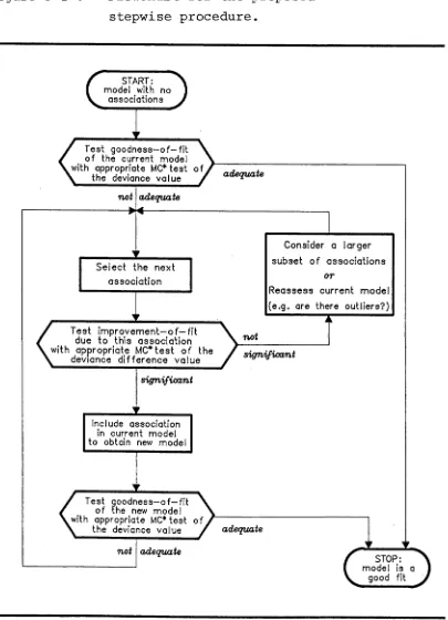
3 . 2 The p r o p o s e d s t e p w i s e p r o c e d u r e .
The sequence of steps for the proposed stepwise procedure for the detection of nonrandom allelic
association using log-linear model analysis is indicated in the flowchart given in figure 3-1.
Figure 3-1 Flowchart for the proposed stepwise procedure.
26 .
f Test goodness—o f —fit ^
of the current model with appropriate MC* test of
V the deviance value > adequate
adequate
Test i m p r o v e m e n t - o f - f i t due to this association with appropriate MC* te s t of the
k deviance differe nce value s ig n ifican t
sig n ifican t
' Test goodness—o f —fit ^
of the new model with appropriate MC* test of
V the deviance value / adequate
adequate
STOP: model is a
good fit Select the next
association
Include association in current model to obtain new model
Reassess current model (e.g. are there outliers?)
Consider a larger subset o f associations
[image:33.557.91.496.132.692.2]2 7.
frequencies) but no parameters for associations between the loci. This is the natural model to start with since interest is in the associations.
The choice as to which unselected association is next, is made as follows. A subset of unselected
associations is considered where the subset is determined by requiring the sequence of models considered by the
stepwise procedure to be nested. To each of these associations is attached an approximate p-value. This P-value is the probability of observing a chi-squared variate as large or larger than the observed deviance difference statistic where the chi-square has degrees of freedom equal to the number of parameters in the
parameterisation of the association. The chosen association is that with the smallest p-value. This selection of the next association is based only on
statistical criteria (smallest p-value). An alternative selection procedure is to choose a smaller subset of unselected associations if the researcher decided that
certain associations in the above (larger) subset should be considered first based on biological criteria, such as
28 .
figure 3-2 for the detection of nonrandom allelic association between four loci (here labelled A,B,C,D)
in the sample from site 8 of the wild barley data referred to in chapter 2.
In figure 3-2 a 'step' roughly refers to the
sequence • choose the next association, test its
improvement-of-fit, test the goodness-of-fit of the new model. Each model is described by the associations it
includes. Below each model description shown are the observed deviance statistic for the model, the
corresponding degrees of freedom and (in brackets) the ranking of this observed deviance statistic in the appropriate Monte Carlo test (where a goodness-of-fit test was required). The models are arranged so that on reading left to right, models with fewer associations
are encountered before those with more. Lines join models for which the right hand model differs from the left
hand model only by the addition of an association. In italics above each line are the deviance difference statistic for the pair of models, the corresponding
degrees of freedom and an approximate P-value as described earlier. The sequence of models chosen by the stepwise procedure is indicated by the thicker lines. At each step the subset of associations shown is the larger subset
determined only on statistical criteria as described earlier.
If, for example, it was known that A,B,C were on one chromosome and D was on another then an appropriate smaller subset of associations at step 1 might be
A .B 8 0 .9 ; 9 5
2 9.
Pig' Qirs 3 - 2 : An e x a m p l e s h o w i n g t h s s t s p w i s s
p r o c e d u r e f o r d e t e c t i n g n o n r a n d o m
a l l e l i c a s s o c i a t i o n .
CD q q
< ä *
5-< rO CD
ä “ < ° ^ < ä
-0 0
q 05 0 o CD o cq < + q o LO oo_ oq CM S--H» 00
o m m “
i o
o 1 0
s « q < cn o uO go iq 00 r-«I -C
n O co ^ rO " "
3 0.
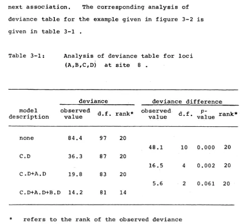
next association. The corresponding analysis of deviance table for the example given in figure 3-2 is
given in table 3-1 .
Table 3-1: Analysis of deviance table for loci (A,B,C,D) at site 8 .
model description
deviance deviance difference
observed
value d.f. rank*
observed
value d.f. valuep" rank*
none 84.4 97 20
48.1 10 0.000 20
C.D 36.3 87 20
16.5 4 0.002 20
C .D+A.D 19.8 83 20
5.6 2 0.061 20
C.D+A.D+B.D 14.2 81 14
refers to the rank of the observed deviance
(deviance difference) statistic in the appropriate Monte Carlo goodness-of-fit (improvement-of-fit) test.
It may occur that the current model is not a 'good fit'
of the data and yet the next association does not give a significant improvement-of-fit result. (In this context it is assumed that the larger subset, described above, is
being considered.) Here it is suggested that the current model should be reassessed.The problem may be caused by,
for example, outliers in the data or the invalidity of
[image:37.557.59.536.66.511.2]3 1.
the distributional assumptions, and so on. Methods described by, for example, Andrews and Pregibon (1978), Dempster and Gasko-Green (1981) and Atkinson (1983)
could be useful here.
This is a stepwise forward selection procedure and carries the usual caveates for such procedures. Any specific stepwise procedure may not lead to a subset of associations which formsan optimal model for the data.
(Here, an optimal model is defined as a model with as few associations as required to provide a good fit and has the
smallest observed deviance statistic of all such models.) However, Furnival-Wilson algorithms (Furnival and Wilson,
1974) and other techniques suggested for selecting the optimal subset of associations (see, for example,
Hocking, 1976) were difficult to implement in the context of log-linear models for multilocus data because of the size and sparsity of the contingency tables involved. The choice of forward selection rather than backward elimination was also because of the size and sparsity of the contingency tables involved which led to numerical instabilities in the fitting procedure when a maximal model containing all possible associations was fitted.
3 . 3 A p p l i c a t i o n o f t h i s s t e p w i s e p r o c e d u r e to
b a r l e y d a t a .
3 2 .
In Part A the analysis was restricted to detecting
nonrandom allelic associations between the loci
Al, Bl, B2, B3, Cl (these five loci being chosen because
they were the most polymorphic loci over all twenty-six sites). This restriction avoided the very large contingency tables encountered when all nineteen loci
were utilised. In the stepwise procedure,selection of the
next association gave preference to those associations between loci on the same chromosome. The results from the analysis of each of the twenty-six sites are given as
analysis of deviance tables in section A.l of the appendix. A summary of these results is given in
figure 3-3.
In figure 3-3 the detected nonrandom allelic
association is depicted at each sampling site. Loci with codes prefixed by the same letter are on the same
chromosome. At each site only those loci which are
polymorphic at that site are shown. For those associations detected the strength of the association is indicated by the thickness of the lines joining the loci involved.
(The strength was judged by the P-value of the deviance difference statistic for the association; the smaller
the p-value the stronger the association and, consequently, the thicker the line.) Broken lines indicate a choice of
associations could be made. No nonrandom allelic association between three or more loci was detected.
An overall biological interpretation of the results given in figure 3-3 is difficult without further knowledge
For example, the consistency of
associations between loci 3 2 and Cl in sites 5, 6 and 8 suggests thele^may be. fror^ the same population & J :cLi£rorv'
populations sharing a common ancestor, an observation Alost
using the measure of Brown et al. However, in comparison
with D statistics some information has been lost. For
3 3.
these data, and this is beyond the scope of this thesis. For comparative purposes the results given by
Brown et a l. (1980) for their analyses of pairwise
nonrandom allelic association at each site are indicated in figure 3-3. These analyses used the summary measure of pairwise nonrandom allelic association as described in Brown et at. and utilised nineteen loci rather than five. Sites at which pairwise nonrandom allelic association was detected are indicated by the pear-shaped backgrounds having solid colour while those sites where no evidence of association was detected have a cross-hatched
background. In most cases the results of part A and those
t.«. ioi/'j- 3*3 -th ots si-tts u / / V A hrk^rouAdZ have artnds-/- one jlAe ( . o s d a t f y ) joining m i
of Brown et al. essentially agree; an exception being site 2 . What is apparent is the difference between the two analyses in the amount of information available
regarding the possible structure of the nonrandom allelic association detected.
In part B the stepwise procedure was used to detect nonrandom allelic association between the nineteen loci used by Brown et al. The numerical problems involved with analysing very large contingency tables restricted analysis in part B to nine sites at which there were five to seven polymorphic loci. The corresponding nine analysis of deviance tables are given in section A.2
of the appendix. A suitable presentation of the detected nonrandom allelic association at any one site is shown in figure 3-4.
3 4 .
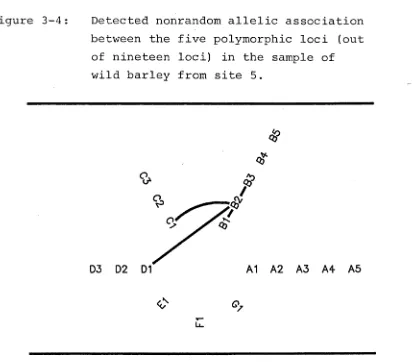
Figure 3-4: Detected nonrandom allelic association between the five polymorphic loci (out
of nineteen loci) in the sample of wild barley from site 5.
D3 D2 D1 A1 A2 A3 A4 A5
<
2,
Those loci which were polymorphic at the particular site are indicated in bold. Loci on the same chromosome begin with the same letter and are shown on the same radius of the circle. The size of this format suggests that a presentation of the results for all the sites analysed, similar to that given in figure 3-3, would be so large as to be cumbersome and therefore has not been given here.
For the purposes of comparison the results from part A (only the loci Al, Bl, B2, B3, Cl) and part B
[image:44.557.84.497.86.448.2]3 5 .
Figure -5: Detected n o n r a n d o m allelic association in
part A (loci Al, Bl, B2, B3, Cl), and
part B (nineteen loci) for each of the
nine sites anal y s e d in part B.
(Results for part A are given first.)
site
2
4
5
8
10
A1
A-1 A.2
B T 1 2 B 3 B.1 B.? B 3
A 1 --- B'2 B 3 c'1
A1 1 A 3| - - - - B 2 B 3 01
I
1
A1 eO T bO
I
C1
A1 01
A1 B2 B3
1 C1
A1 A2 _B? B 3 C1
lr
A1 B2 b'5 ---- >C1l
A1 A3
l_ B2 B3 C11
AI Bl B2 B3 C1
A1__A2____ A5 Bl B2 B3 C1
18
19
20
A1
A1 A2 A5
B2
B2
C1
Cl 02
A1 B2_ B3 C11
AI A2 A5 B2 B3
L 1 C1
A1 B2~B3 C1
AI A2 A5 B2 B3 01 02l__1
36 .
In figure 3-5 lines join loci between which nonrandom allelic association was detected. For each site the
results for part A are shown first and only those loci which were polymorphic and therefore relevant to the
analysis are shown. For some sites (for example, 2 and 20) the structure of the detected nonrandom allelic
associations between the loci analysed in part A were
essentially unaltered by the incorporation of further loci into the analysis while for other sites (for example,
5 and 19) there were substantial alterations. This suggests that, in general, caution is required when
'pooling' multilocus gametic data. This agrees with the observation that 'pooling' data obscures possible
nonrandom allelic association (Langley.et al. 3 (1974),
Zouros, Golding and MacKay, 1977; Weir and Cockerham, 1978). In summary these results show the usefulness of
this approach to detecting nonrandom allelic association in providing a possible structure of the detected nonrandom allelic association. However, as shown by only nine sites being analysed in part B , the approach can suffer
3 7.
3.4. E m p i r i c a l r e s u l t s f o r t h e t e s t p r o c e d u r e s d i s c u s s e d in s e c t i o n 3 . 1 .
The results in this section concern the properties
of the test procedures used in the log-linear model analysis and were obtained concurrently with the analysis of the
wild barley data described in section 3.3. The models used are listed in section A.3 of the appendix together with characteristics of the data sets utilised for the
simulations.
The first results given show how the usual chi-squared approximations for the empirical sampling distributions
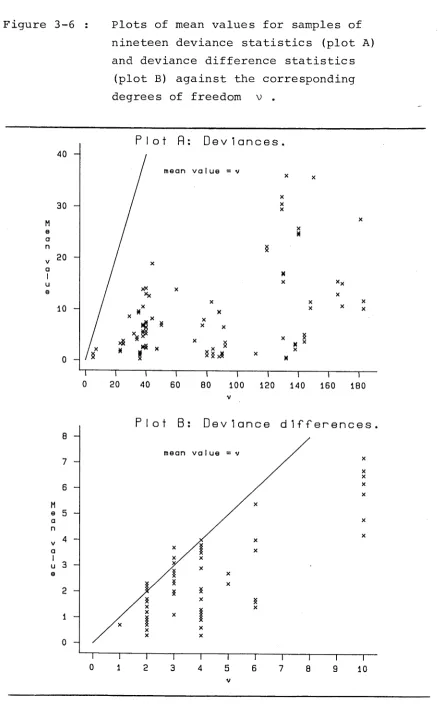
of the deviance and deviance difference statistics are inappropriate. In figure 3-6 are plots of 104 mean values for samples of nineteen deviance statistics
(plot A) and 65 mean values for samples of nineteen deviance difference statistics (plot B) against the corresponding degrees of freedom v .
In both plots many of the mean values are well
below their corresponding value of v . For the deviance statistic a trend was noted for mean values to be further from their corresponding values of v as the percentage of cells with zero frequencies increased. However, no function involving these percentages or other
characteristics of the data or the model could be
determined such that more appropriate values of v could
be suggested.
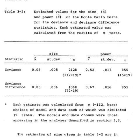
In table 3-2 are the estimated values of the size
CD
C
3 8.
Figure 3-6 : Plots of mean values for samples of nineteen deviance statistics (plot A) and deviance difference statistics
(plot B) against the corresponding degrees of freedom v .
Plot fl D e v i a n c e s
mean value
D e v i a n c e d i f f e r e n c e s
[image:48.557.75.513.64.768.2]3 9
.
in section 3.1 for the deviance and deviance difference statistics.
Table 3-2: Estimated values for the size (a)
A
and power (t t) of the Monte Carlo tests for the deviance and deviance difference statistics. Each estimated value was calculated from the results of n tests.
size power
statistic aA st.dev. n
A
TT st.dev. n
[image:49.557.56.512.120.594.2]deviance 0.05 .005 2128
(112x19)*
0.52 .017 855
(45x19)
deviance
difference 0.05 .006 1368
(72x19)
0.67 .016 855
* Each estimate was calculated from m (=112, here)
choices of model and data each of which was simulated 19 times. The models and data chosen were those appearing in the analyses described in section 3.3.
The estimates of size given in table 3-2 are in
agreement with the Monte Carlo test procedure having exact size a =0.05 as suggested by Hope (1968) . The
estimates of power are within the range suggested by Marriott (1979) as the power range for Monte Carlo tests using = 1 . Further examination of the results of
4 0.
PART II
Multilocus Data in Medical Genetics
C H A P T E R 4
D E T E C T I N G N O N R A N D O M A L L E L I C A S S O C I A T I O N IN
M U L T I L O C U S G E N O T Y P I C D A T A
4. 1 I n t r o d u c t i o n .
Multilocus data of the form usually collected in medical studies is the primary concern of this second part
of the thesis. Typically, in medical studies the
constituent gametes of the diploid individuals cannot be determined. Data of this form will be termed genotypic
data as distinct from gametic data in which the constituent gametes are known.
This chapter considers the detection of nonrandom allelic association in multilocus genotypic data measured at a population level. The main aspects of methods usually employed for data on two loci in a randomly mating
population have been developed and discussed by, for
4 1.
Smouse (1974) and Hill (1975) described approaches to the
analysis of multiple loci but they still assumed random mating in the population. All of these methods assume gametic frequencies are available either through direct observation or via maximum likelihood estimation assuming a random mating population. Tests for, and measures of, nonrandom allelic association could then be based on these gametic frequency estimates. These methods based on first obtaining gametic frequencies may be inapplicable.
Some species are not amenable to techniques, such as progeny testing, used to apportion double heterozygotes to coupling and repulsion phases thus precluding the direct observation of constituent gamete types. The usual
alternative has been to employ maximum likelihood
estimation to obtain estimates of the gametic frequencies from the observed genotypic frequencies. However, should deviations from Hardy-Weinberg equilibrium be present then these maximum likelihood methods may give incorrect
estimates for the gametic frequencies.
For analysis in these situations composite measures of nonrandom allelic association, involving sums of
intra-gametic and inter-gametic association, have been developed for the two locus situation (Weir and Cockerham,
1979, and Weir, 1979). Haber (1984) combines a log-linear model analysis with the EM algorithm to obtain tests of
4 2.
choice of models for the data. However, this iterative approach may contain undetected convergence problems.
In this chapter an approach is outlined based on applying the concept of composite link functions to a
log-linear model analysis. Composite link functions were
originally formulated by Thompson and Baker (1981) and have been further examined by Burn (1982), Roger (1983) and Gilchrist (1985). The approach provides tests of
hypotheses concerning random mating and nonrandom allelic associations. Also, genotypic data for multilocus systems can be accommodated and a number of other, useful,
extensions are readily accessible.
A computationally simpler approach to analysing such data is considered in section 4.3. This approach assumes the gametic phases are equiprobable allowing construction of a set of gametic frequencies from the observed
genotypic frequencies. This assumption was used by, for example, Muona (1982) in the analysis of barley data.
The validity of this assumption for human data is evaluated by comparison with the exact results from the
computationally more complex approach using the composite link function. Artificial human genotypic data with known structure are used for the evaluation.
4 . 2 T h e c o m p o s i t e l i n k f u n c t i o n a p p r o a c h .
Consider genotypic data for individuals in a diploid
population with alleles at the ith locus,
i = l,...,Af . The observed data consist of the
4 3.
genotypic data the different forms of analogous multiple heterozygotes cannot be distinguished. Consequently, the observed genotypic data vector, y , of length
A
M H i
IK = 1 [A ^ + (2 )) has to be considered as being derived
from an unobserved gametic data vector, z , of length
( I A/) 2 . To illustrate this consider two loci,
locus 1 with alleles £ {X,Y} , locus 2 with alleles
k,£ and assume codominance. The relationship between the 9 observable genotypic frequencies,
yijki r and the 16 unobservable gametic frequencies,
ik
z . , can be obtained from figure 4-1 by relating each J ^
cell frequency, ik
zjl ’ as indicated.
Figure 4-1:
z i k
3£
w w
k £
wz zw ZZ
XZ
yxxww y xxwz yxxzz
XY
YX yXYWW y XYWZ yXYZZ
YY
y YYWW y YYWZ y YYZZ
Let y represent the observed genotypic
frequency of individuals having genotype ijkZmn...
where tJt/ are the two alleles appearing at locus 1 , ^ Jc in
k , £ at locus 2 and so on. Let z.Q **’ represent the gametic frequency of the type ikm.../jin... where
4 4.
in one constituent gamete and j,£,n,... are the alleles appearing at loci 1,2,3,... in the other.
The mapping from the gametic data vector to the observed genotypic data vector can be written as
(4.1)
yijkZmn... E .
a , b e {i , j } a ,d E ik , £}
e ,f E im ,n}
ace , ''bdf.
For example, in figure 4-1, yxxww = zx w > X W X z
yxxwz = ZXZ + ZXW an<^ 1***S° °n * In m a t r ^x f°rm equation (4.1) appears as
(4.2) y = Cz
where C is the appropriate matrix (of elements 1 and
A
M i M
0) having size n^_^(^4^.+ ( ^)) x ( I T . In particular, for the example given in figure 4-1
C
1 0 0 0 0 0 1 1 0 0 0 0 0 1 0 0 0 0 0 1 0 0 0 0 0 0 0 0 0 0 0 0 0 0 0 0 0 0 0 0
^ 0 0 0 0 0
0 00 0 0 0
0 00 0 0 0 0 00 0 0 0 0 00 1 0 0 1 1 0 O i l
0 01 0 0 0 0 00 0 0 0 0 0 0 0 0 0 0 00 0 0 0
0 0 0 0 0
0 0 0 0 0
0 0 0 0 0
4 5.
Let Y be the vector of e x pected gametic frequencies
c o r r e s p o n d i n g to the gametic frequencies z . The most
general log-linear model of immediate biological relevance
for the expe c t e d gametic frequencies is
(4.3) In i k m...
^ jZn. . . y +
E
aa+ E
be E { i j rk Z , m n,...} be
+ ,
E
de G { i k Z , i m , j n , k m ,Zn
+ E
e ii Z , jk , in , jm ,kn , Zm
e de
..} 5
The parameters depend on the relative
frequencies of the individual alleles. The parameters (j),
be
measure deviations from H a r d y - W e i n b e r g equilibrium. The
p a rameters m e a sure intra-gametic non r a n d o m allelic
association between pairs of loci while the 6^ param e t e r s
measure the c o r r e s p o n d i n g inter-gametic nonrandom allelic
association. A cons e q u e n c e of the different forms of
analogous multiple h e t e r o z y g o t e s being indistinguishable
is that in the estim a t i o n the intra-gametic n o n r andom
allelic a s s o ciation terms (s) are c o nfounded with the
inter-gametic n o n r a n d o m allelic association terms (6) .
Extensions to include h igher order n o n random allelic
association involve including further parameters in
equation (4.3) . For example, intra-gametic n o n random