SIEVE INFERENCE ON SEMI-NONPARAMETRIC
TIME SERIES MODELS
By
Xiaohong Chen, Zhipeng Liao and Yixiao Sun
February 2012
COWLES FOUNDATION DISCUSSION PAPER NO. 1849
COWLES FOUNDATION FOR RESEARCH IN ECONOMICS
YALE UNIVERSITY
Box 208281
New Haven, Connecticut 06520-8281
http://cowles.econ.yale.edu/
Sieve Inference on Semi-nonparametric Time Series Models
Xiaohong Cheny, Zhipeng Liaoz, and Yixiao Sunx
First Draft: October 2009; This draft: February 2012
Abstract
The method of sieves has been widely used in estimating semiparametric and nonparametric models. In this paper, we …rst provide a general theory on the asymptotic normality of plug-in sieve M estimators of possibly irregular functionals of semi/nonparametric time series models. Next, we establish a surprising result that the asymptotic variances of plug-in sieve M estimators of irregular (i.e., slower than root-Testimable) functionals do not depend on temporal dependence. Nevertheless, ignoring the temporal dependence in small samples may not lead to accurate inference. We then propose an easy-to-compute and more accurate inference procedure based on a “pre-asymptotic” sieve variance estimator that captures temporal dependence. We construct a “pre-asymptotic”Wald statistic using an orthonormal series long run variance (OS-LRV) estimator. For sieve M estimators of both regular (i.e., root-T estimable) and irregular functionals, a scaled “pre-asymptotic” Wald statistic is asymptoticallyF distributed when the series number of terms in the OS-LRV estimator is held …xed. Simulations indicate that our scaled “pre-asymptotic”Wald test withF critical values has more accurate size in …nite samples than the usual Wald test with chi-square critical values.
Keywords: Weak Dependence; Sieve M Estimation; Sieve Riesz Representor; Irregular Functional; Misspeci…cation; Pre-asymptotic Variance; Orthogonal Series Long Run Variance Estimation; F Distribution
We acknowledge useful comments from T. Christensen, J. Hahn, L. Hansen, J. Hidalgo, M. Jansson, D. Kaplan, O. Linton, P. Phillips, D. Pouzo, J. Powell, H. White, and other participants at 2011 Econometrics Society Australasian Meeting in Adelaide, the Pre-conference Workshop of 2011 Asian Meeting of the Econometric Society in Seoul, econo-metrics workshops at Yale, UC Berkeley, UCLA, UCSD and Stanford. Chen and Sun acknowledge …nancial support from the National Science Foundation under the respective grant numbers: SES-0838161 and SES-0752443. Any errors are the responsibility of the authors.
yDepartment of Economics, Yale University, 30 Hillhouse, Box 208281, New Haven, CT 06520. Email: [email protected]
zDepartment of Economics, UC Los Angeles, 8379 Bunche Hall, Mail Stop: 147703, Los Angeles, CA 90095. Email: [email protected]
1
Introduction
Many economic and …nancial time series (and panel time series) are nonlinear and non-Gaussian; see, e.g., Granger (2003). For policy and welfare analysis, it is important to uncover complicated nonlinear economic relations in dynamic structural models. Unfortunately, it is di¢ cult to correctly parameterize nonlinear dynamic functional relations. Even if the nonlinear functional relation among the observed variables is correctly speci…ed by economic theory or by chance, misspecifying distributions of nonseparable latent variables could lead to inconsistent estimates of structural parameters of interest. These reasons, coupled with the availability of larger data sets, motivate the growing popularity of semiparametric and nonparametric models and methods in economics and …nance.
The method of sieves (Grenander, 1981) is a general procedure for estimating semiparametric and nonparametric models, and has been widely used in economics, …nance, statistics and other disciplines. In particular, the method of sieve extremum estimation optimizes a random criterion function over a sequence of approximating parameter spaces, sieves, that becomes dense in the original in…nite dimensional parameter space as the complexity of the sieves grows to in…nity with the sample size T. See, e.g., Chen (2007, 2011) for detailed reviews of some well-known empirical applications of the method and existing theoretical properties of sieve extremum estimators.
In this paper, we consider inference on possibly misspeci…ed semi-nonparametric time series models via the method of sieves. We focus on sieve M estimation, which optimizes a sample average of a criterion function over a sequence of …nite dimensional sieves whose complexity grows to in…nity with the sample sizeT. Prime examples include sieve quasi maximum likelihood, sieve (nonlinear) least squares, sieve generalized least squares, and sieve quantile regression. For general sieve M estimators with weakly dependent data, White and Wooldridge (1991) establish the consistency, and Chen and Shen (1998) establish the convergence rate and thepT asymptotic normality of plug-in sieve M estimators of regular (i.e., pT estimable) functionals. To the best of our knowledge, there is no published work on the limiting distributions of plug-in sieve M estimators of irregular (i.e., slower thanpT estimable) functionals. There is also no published inferential result for general sieve M estimators of regular or irregular functionals for possibly misspeci…ed semi-nonparametric time series models.
We …rst provide a general theory on the asymptotic normality of plug-in sieve M estimators of possibly irregular functionals in semi/nonparametric time series models. This result extends that of Chen and Shen (1998) for sieve M estimators of regular functionals to sieve M estimators of irregular functionals. It also extends that of Chen and Liao (2008) for sieve M estimators of irregular functionals with iid data to time series settings. The asymptotic normality result is rate-adaptive in the sense that researchers do not need to knowa priori whether the functional of interest ispT estimable or not.
For weakly dependent data and for regular functionals, it is known that the asymptotic variance expression depends on the temporal dependence and is usually equal to the long run variance (LRV) of
a scaled moment (or score) process. It is often believed that this result would also hold for sieve esti-mators of irregular functionals such as the evaluation functionals and weighted integration functionals. Contrary to this common belief, we show that under some general conditions the asymptotic variance of the plug-in sieve estimator for weakly dependent data is the same as that for iid data. This is a very surprising result, as sieve estimators are often regarded as global estimators, and hence autocorrelation is not expected to vanish in the limit (asT ! 1).
Our asymptotic theory suggests that, for weakly dependent time series data with a large sam-ple size, temporal dependence could be ignored in making inference on irregular functionals via the method of sieves. This resembles the earlier well-known asymptotic results for time series density and regression functions estimated via kernel and local polynomial regression methods. See, e.g., Robinson (1983), Fan and Yao (2003), Li and Racine (2007), Gao (2007) and the references therein. However, simulation studies indicate that inference procedures based on asymptotic variance estimates ignoring autocorrelation may not perform well when the sample size is small (relatively to the degree of temporal dependence). See, e.g., Conley, Hansen and Liu (1997) and Pritsker (1998) for earlier discussion of this problem with kernel density estimation for interest rate data sets.
In this paper, for both regular and irregular functionals of semi-nonparametric time series models, we propose computationally simple, accurate and robust inference procedures based on estimates of “pre-asymptotic”sieve variances capturing temporal dependence. That is, we treat the underlying triangular array sieve score process as a generic time series and ignore the fact that it becomes less temporally dependent when the sieve number of terms in approximating unknown functions grows to in…nity asT goes to in…nity. This “pre-asymptotic” approach enables us to conduct easy-to-compute and accurate inference on semi-nonparametric time series models by adopting any existing autocorrelation robust inference procedures for (misspeci…ed) parametric time series models.
For semi-nonparametric time series models, we could compute various “pre-asymptotic” Wald sta-tistics using various existing LRV estimators for regular functionals of (misspeci…ed) parametric time series models, such as the kernel LRV estimators considered by Newey and West (1987), Andrews (1991), Jansson (2004), Kiefer and Vogelsang (2005), Sun (2011b) and others. Nevertheless, to be consistent with our focus on the method of sieves and to derive a simple and accurate asymptotic approximation, we compute a “pre-asymptotic” Wald statistic using an orthonormal series LRV (OS-LRV) estimator. The OS-LRV estimator has already been used in constructing autocorrelation robust inference on regular functionals of parametric time series models; see, e.g., Phillips (2005), Müller (2007), Sun (2011a), and the references therein. We extend these results to robust inference on both regular and irregular functionals of semi-nonparametric time series models.1
For both regular and irregular functionals, we show that the “pre-asymptotic”tstatistic and a scaled
1
We thank Peter Phillips for suggesting that we consider autocorrelation robust inference for semi-nonparametric time series models.
Wald statistic converge to the standardtdistribution and F distribution respectively when the series number of terms in the OS-LRV estimator is held …xed; and that thetdistribution andF distribution approach the standard normal and chi-square distributions respectively when the series number of terms in the OS-LRV estimator goes to in…nity. Our “pre-asymptotic”tandF approximations achieve triple robustness in the following sense: they are asymptotically valid regardless of (1) whether the functional is regular or not; (2) whether there is temporal dependence or not; and (3) whether the series number of terms in the OS-LRV estimator is held …xed or not.
To facilitate the practical use of our inference procedure, we show that, in …nite samples and for linear sieve M estimators, our “pre-asymptotic” sieve test statistics (i.e. t statistic and Wald statistic) for semi-nonparametric time series models are numerically equivalent to the corresponding test statistics one would obtain if the models are treated as if they were parametric.2 These results are of much use to applied researchers, and demonstrate the advantage of the sieve method for inference on semi-nonparametric time series models.
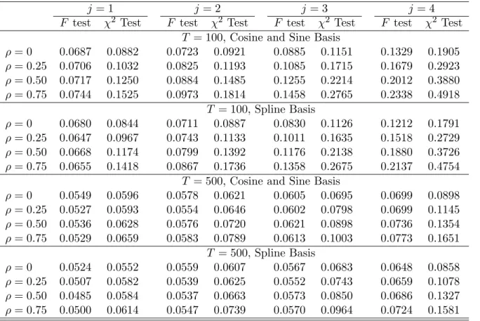
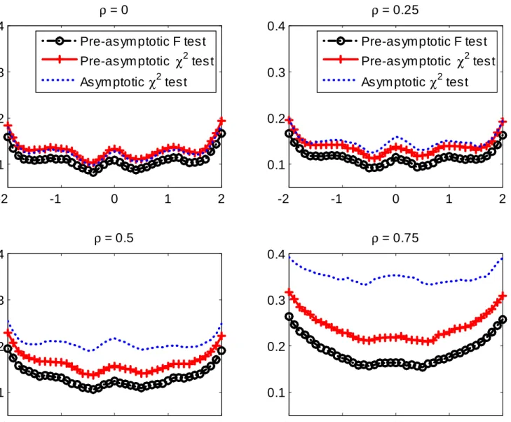
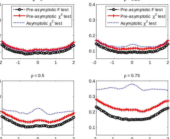
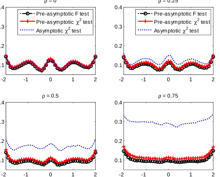
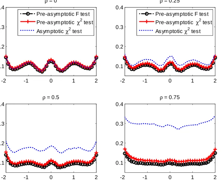
To investigate the …nite sample performance of our proposed “pre-asymptotic” robust inference procedures on semi-nonparametric time series models, we conduct a detailed simulation study using a partially linear regression model. For both regular and irregular functionals, we …nd that our test using the “pre-asymptotic” scaled Wald statistic and F critical values has more accurate size than the “pre-asymptotic” Wald test using chi-square critical values. For irregular functionals, we …nd that they both perform better than the Wald test using a consistent estimate of the asymptotic variance ignoring autocorrelation. These are especially true when the time series (with moderate sample size) has strong temporal dependence and the number of joint hypotheses being tested is large. Based on our simulation studies, we recommend the use of the “pre-asymptotic” scaled Wald statistic using an OS-LRV estimator andF approximation in empirical applications.
The rest of the paper is organized as follows. Section 2 presents the plug-in sieve M estimator of functionals of interest and gives two illustrative examples. Section 3 establishes the asymptotic normality of the plug-in sieve M estimators of possibly irregular functionals. Section 4 shows the surprising result that the asymptotic variances of plug-in sieve M estimators of irregular functionals for weakly dependent time series data are the same as if they were for i.i.d. data. Section 5 presents the “pre-asymptotic”OS-LRV estimator andF approximation. Section 6 proves the numerical equivalence result. Section 7 reports the simulation evidence, and the last section brie‡y concludes. Appendix A contains all the proofs, and Appendix B discusses the properties of the hidden delta functions associated with sieve M estimation of evaluation functionals.
Notation. In this paper, we denote fA(a) (FA(a)) as the marginal probability density (cdf) of
2
Here we slightly abuse terminology and de…ne a parametric model to be a model with a …xed …nite number of unknown parameters of interest, although the model may contain in…nite dimensional nuisance parameters that are not needed to be estimated, such as Hansen (1982)’s GMM models.
a random variable A evaluated at a and fAB(a; b) (FAB(a; b)) the joint density (cdf) of the random
variables A and B. We use to introduce de…nitions. For any vector-valued A, we let A0 denote its transpose and jjAjjE
p
A0A, although sometimes we also use jAj = pA0A without too much
confusion. Denote Lp( ; d ), 1 p < 1, as a space of measurable functions with jjgjjLp( ;d )
fR jg(t)jpd (t)g1=p <1, where is the support of the sigma-…nite positive measure d (sometimes Lp( )and jjgjjLp( ) are used when d is the Lebesgue measure). For any (possibly random) positive
sequencesfaTg1T=1 and fbTg1T=1, aT =Op(bT) means that limc!1lim supTPr (aT=bT > c) = 0;aT =
op(bT) means that for all " >0, limT!1Pr (aT=bT > ") = 0; andaT bT means that there exist two
constants0< c1 c2 <1 such that c1aT bT c2aT. We useAT AkT, HT HkT andVT VkT
to denote various sieve spaces. To simplify the presentation, we assume that dim(VT) = dim(AT) dim(HT) kT, all of which grow to in…nity with the sample size T.
2
Sieve M Estimation and Examples
2.1 Basic Setting
We assume that the datafZt= (Yt0; Xt0)0gTt=1 is from a strictly stationary and weakly dependent process
de…ned on an underlying complete probability space. Let the support ofZt be Z Rdz;1 dz <1,
and letY and X be the supports of Y and X respectively. Let (A; d) denote an in…nite dimensional metric space. Let `:Z A !R be a measurable function and E[`(Z; )] be a population criterion. For simplicity we assume that there is a unique 0 2(A; d) such that E[`(Z; 0)]> E[`(Z; )] for all 2 (A; d) with d( ; 0) > 0. Di¤erent models in economics correspond to di¤erent choices of the criterion functionsE[`(Z; )] and the parameter spaces(A; d). A model does not need to be correctly speci…ed and 0 could be a pseudo-true parameter. Let f : (A; d) ! R be a known measurable
mapping. In this paper we are interested in estimation of and inference on f( 0) via the method of
sieves.
LetAT be a sieve space for the whole parameter space(A; d). Then there is an element T 0 2 AT
such thatd( T 0; 0)!0 as dim(AT) ! 1(with T). An approximate sieve M estimator bT 2 AT
of 0 solves 1 T T X t=1 `(Zt;bT) sup 2AT 1 T T X t=1 `(Zt; ) Op("2T); (2.1)
where the term Op("2T) = op(T 1) denotes the maximization error when bT fails to be the exact
maximizer over the sieve space. We callf(bT) theplug-in sieve M estimator of f( 0).
Under very mild conditions ( see, e.g., Chen (2007, Theorem 3.1) and White and Wooldridge (1991)), the sieve M estimator bT is consistent for 0: d(bT; 0) = Opfmax [d(bT; T 0); d( T 0; 0)]g =
2.2 Examples
The method of sieve M estimation includes many special cases. Di¤erent choices of criterion functions `(Zt; ) and di¤erent choices of sieves AT lead to di¤erent examples of sieve M estimation. As an
illustration, we provide two examples below. See, e.g., Chen (2007, 2011) for additional applications.
Example 2.1 (Partially linear ARX regression) Suppose that the time series data fYtgTt=1 is
generated by
Yt=X1;t0 0+h0(X2;t) +ut; E[utjX1;t; X2;t] = 0; (2.2)
where X1;t and X2;t are d1 and d2 dimensional random vectors respectively, and X1;t could include
…nitely many lagged Yt’s. Let 0 2 Rd1 and h0 2 H a function space. Let 0 = ( 00; h0)0 2 A = H. Examples of functionals of interest could be f( 0) = 0 0 or h0(x2) where 2Rd1 and x2 is
some point in the support ofX2;t.
LetXj be the support ofXj forj = 1;2. For simplicity we assume thatX2 is a convex and bounded
subset ofRd2. For the sake of concreteness we letH= s(X
2)(a Hölder space): s( X2) = ( h2C[s](X2) : sup j [s] sup x2X2 h(j)(x) <1; sup x;x02X2 h([s])(x) h([s])(x0) jx x0js [s] <1 ) ;
where[s]is the largest integer that is strictly smaller thans. The Hölder space s(X2)(withs >0:5d2)
is a smooth function space that is widely assumed in the semi-nonparametric literature. We can then approximateH= s(X2) by various linear sieve spaces:
HT = 8 < :h( ) :h( ) = kT X j=1 jpj( ) = 0PkT( ); 2R kT 9 = ;; (2.3)
where the known sieve basis PkT( ) could be tensor-products of splines, wavelets, Fourier series and
others; see, e.g., Newey (1997) and Chen (2007). Let`(Zt; ) = Yt X1;t0 h(X2;t)
2
=4withZt= (Yt; X1;t0 ; X2;t0 )0 and = ( 0; h)0 2 A= H.
LetAT = HT be a sieve forA. We can estimate 0= ( 00; h0)0 2 Aby the sieve least squares (LS)
(a special case of sieve M estimation):
bT (bT0 ;bhT)0 = arg max ( ;h)2 HT 1 T T X t=1 `(Zt; ; h). (2.4)
A functional of interest f( 0) (such as 0 0 or h0(x2)) is then estimated by the plug-in sieve LS
estimatorf(bT) (such as 0bT orbhT (x2)).
This example is very similar to example 2 in Chen and Shen (1998) and example 4.2.3 in Chen (2007). One can slightly modify their proofs to get the convergence rate of bT and the
p
normality of 0bT. But neither paper provides a variance estimator for 0bT. The results in our paper
immediately lead to the asymptotic normality of f(bT) for possibly irregular functionals f( 0) and
provide simple, accurate inference onf( 0).
Example 2.2 (Possibly misspeci…ed copula-based time series model) Suppose that fYtgTt=1 is
a sample of strictly stationary …rst order Markov process generated from(FY; C0(; )), whereFY is the
true unknown continuous marginal distribution, and C0(; ) is the true unknown copula for (Yt 1; Yt)
that captures all the temporal and tail dependence of fYtg. The -th conditional quantile of Yt given
Yt 1 = (Y
t 1; :::; Y1) is:
QY(y) =FY 1 C2j11[ jFY(y)] ;
whereC2j1[ju] @u@ C0(u; )is the conditional distribution ofUt FY(Yt)givenUt 1 =u, andC2j11[ ju]
is its -th conditional quantile. The conditional density function ofYt given Yt 1 is
p0(jYt 1) =fY( )c0(FY(Yt 1); FY( ));
wherefY( )andc0(; )are the density functions ofFY( )andC0(; ) respectively. A researcher speci…es
a parametric formfc(; ; ) : 2 g for the copula density function, but it could be misspeci…ed in the sensec0(; )2 f= c(; ; ) : 2 g. Let 0 be the pseudo true copula dependence parameter:
0= arg max 2 Z 1 0 Z 1 0 c(u; v; )c0(u; v)dudv.
Let ( 00; fY)0 be the parameters of interest. Examples of functionals of interest could be 0 0, fY (y),
FY (y) or QY0:01(y) =FY1 C 1
2j1[ jFY(y); 0] for any 2R
d and somey
2supp(Yt).
We could estimate( 00; fY)0 by the method of sieve quasi ML using di¤erent parameterizations and
di¤erent sieves for fY. For example, let h0 =pfY and 0 = ( 00; h0)0 be the (pseudo) true unknown
parameters. Then fY ( ) =h20( )= R1
1h20(y)dy, andh0 2L2(R). For the identi…cation of h0, we can
assume thath0 2 H: H= 8 < :h( ) =p0( ) + 1 X j=1 jpj( ) : 1 X j=1 2 j <1 9 = ;; (2.5)
where fpjg1j=0 is a complete orthonormal basis functions in L2(R), such as Hermite polynomials,
wavelets and other orthonormal basis functions. Here we normalize the coe¢ cient of the …rst basis functionp0( )to be 1in order to achieve the identi…cation ofh0( ). Other normalization could also be
used. It is now obvious thath02 H could be approximated by functions in the following sieve space:
HT = 8 < :h( ) =p0( ) + kT X j=1 jpj( ) =p0( ) + 0PkT( ) : 2R kT 9 = ;: (2.6)
LetZt0= (Yt 1; Yt), = ( 0; h)02 A= H and `(Zt; ) = log ( h2(Y t) R1 1h2(y)dy ) + log ( c Z Yt 1 1 h2(y) R1 1h2(x)dx dy; Z Yt 1 h2(y) R1 1h2(x)dx dy; !) : (2.7)
Then 0 = ( 00; h0)0 2 A= H could be estimated by the sieve quasi MLE bT = (bT0 ;bhT)0 2 AT = HT that solves: sup 2 HT 1 T ( T X t=2 `(Zt; ) + log ( h2(Y1) R1 1h2(y)dy )) Op("2T): (2.8)
A functional of interest f( 0) (such as 0 0, fY (y) = h20(y)= R1
1h20(y)dy, FY (y) or QY0:01(y)) is
then estimated by the plug-in sieve quasi MLE f(bT) (such as 0b, fbY (y) = bh2T (y)= R1 1bh 2 T (y)dy, b FY (y) = Ry 1fbY(y)dyor Qb Y 0:01(y) =Fb 1 Y (C 1 2j1[ jFbY(y);b])).
Under correct speci…cation, Chen, Wu and Yi (2009) establish the rate of convergence of the sieve MLE bT and provide a sieve likelihood-ratio inference for regular functionals includingf( 0) = 0 0 or
FY (y)orQY0:01(y). Under misspeci…ed copulas, by applying Chen and Shen (1998), we can still derive
the convergence rate of the sieve quasi MLE bT and the p
T asymptotic normality off(bT)for regular
functionals. However, the sieve likelihood ratio inference given in Chen, Wu and Yi (2009) is no longer valid under misspeci…cation. The results in this paper immediately lead to the asymptotic normality off(bT) (such asfbY (y) =bh2T (y)=
R1
1bh2T (y)dy) for any possibly irregular functional f( 0) (such as
fY (y)) as well as valid inferences under potential misspeci…cation.
3
Asymptotic Normality of Sieve M-Estimators
In this section, we establish the asymptotic normality of plug-in sieve M estimators of possibly irregular functionals of semi-nonparametric time series models. We also give a closed-form expression for the sieve Riesz representor that appears in our asymptotic normality result.
3.1 Local Geometry
Given the existing consistency result (d(bT; 0) =op(1)), we can restrict our attention to a shrinking
d-neighborhood of 0. We equip Awith an inner product induced normk 0kthat is weaker than
d( ; 0)(i.e.,k 0k cd( ; 0)for a constantc), and is locally equivalent to p
E[`(Zt; 0) `(Zt; )]
in a shrinking d-neighborhood of 0. For strictly stationary weakly dependent data, Chen and Shen
(1998) establish the convergence ratekbT 0k = Op( T) = o T 1=4 . The convergence rate result
implies that bT 2 BT B0 with probability approaching one, where
B0 f 2 A:k 0k C T log(log(T))g; BT B0\ AT: (3.1)
De…ne
0;T arg min
2BTjj
0jj: (3.2)
Let VT clsp(BT) f 0;Tg, where clsp(BT) denotes the closed linear span of BT under k k. Then VT is a …nite dimensional Hilbert space under k k. Similarly the space V clsp(B0) f 0g is a
Hilbert space under k k. Moreover, VT is dense in V under k k. To simplify the presentation, we
assume that dim(VT) = dim(AT) kT, all of which grow to in…nity with T. By de…nition we have h 0;T 0; vTi= 0 for allvT 2 VT.
As demonstrated in Chen and Shen (1998) and Chen (2007), there is lots of freedom to choose such a norm k 0k that is weaker than d( ; 0) and is locally equivalent to
p
E[`(Z; 0) `(Z; )]. In
some parts of this paper, for the sake of concreteness, we present results for a speci…c choice of the norm k k. We suppose that for all in a shrinking d-neighborhood of 0, `(Z; ) `(Z; 0) can be
approximated by (Z; 0)[ 0]such that (Z; 0)[ 0]is linear in 0. Denote the remainder
of the approximation as:
r(Z; 0)[ 0; 0] 2f`(Z; ) `(Z; 0) (Z; 0)[ 0]g: (3.3)
When lim !0[(`(Z; 0 + [ 0]) `(Z; 0))= ] is well de…ned, we could let (Z; 0)[ 0] = lim !0[(`(Z; 0+ [ 0]) `(Z; 0))= ], which is called the directional derivative of `(Z; ) at 0
in the direction[ 0]. De…ne
k 0k= p
E( r(Z; 0)[ 0; 0]) (3.4)
with the corresponding inner producth; i
h 1 0; 2 0i=Ef r(Z; 0)[ 1 0; 2 0]g (3.5)
for any 1; 2 in the shrinking d-neighborhood of 0. In general this norm de…ned in (3.4) is weaker
than d(; ). Since 0 is the unique maximizer of E[`(Z; )] on A, under mild conditions k 0k
de…ned in (3.4) is locally equivalent topE[`(Z; 0) `(Z; )]. For anyv2 V;we de…ne @f( 0)
@ [v]to be the pathwise (directional) derivative of the functionalf( )
at 0 and in the direction ofv= 02 V :
@f( 0)
@ [v] =
@f( 0+ v)
@ =0 for any v2 V: (3.6) For anyvT = T 0;T 2 VT;we let
@f( 0) @ [vT] = @f( 0) @ [ T 0] @f( 0) @ [ 0;T 0]: (3.7) So @f( 0)
Note thatVT is a …nite dimensional Hilbert space. As any linear functional on a …nite dimensional
Hilbert space is bounded, we can invoke the Riesz representation theorem to deduce that there is a vT 2 VT such that @f( 0) @ [v] =hvT; vi for all v2 VT (3.8) and that @f( 0) @ [vT] =kvTk 2 = sup v2VT;v6=0 j@f( 0) @ [v]j 2 kvk2 (3.9)
We callvT thesieve Riesz representor of the functional @f( 0)
@ [ ]on VT.
We emphasize that the sieve Riesz representation (3.8)–(3.9) of the linear functional @f( 0)
@ [ ]onVT
always exists regardless of whether @f( 0)
@ [ ]is bounded on the in…nite dimensional spaceV or not.
If @f( 0)
@ [ ] is bounded on the in…nite dimensional Hilbert spaceV, i.e. kv k sup
v2V;v6=0 j
@f( 0)
@ [v]j=kvk <1; (3.10) then kvTk=O(1) (in factkvTk % kv k<1 and kv vTk !0 as T ! 1); we say that f( )
is regular (at = 0). In this case, we have @f@( 0)[v] =hv ; vi for all v 2 V, andv is the Riesz
representor of the functional @f( 0)
@ [ ]on V.
If @f( 0)
@ [ ] is unbounded on the in…nite dimensional Hilbert spaceV, i.e. sup
v2V;v6=0 j
@f( 0)
@ [v]j=kvk =1; (3.11) then kvTk % 1asT ! 1; and we say thatf( ) isirregular (at = 0).
As it will become clear later, the convergence rate off(bT) f( 0)depends on the order of kvTk.
3.2 Asymptotic Normality
To establish the asymptotic normality off(bT)for possibly irregular nonlinear functionals, we assume: Assumption 3.1 (local behavior of functional)
(i) sup 2BT f( ) f( 0) @f@( 0)[ 0] =o T 1 2 kv Tk ; (ii) @f( 0) @ [ 0;T 0] =o T 1 2 kv Tk :
Assumption 3.1.(i) controls the linear approximation error of possibly nonlinear functionalf( ). It is automatically satis…ed whenf( ) is a linear functional, but it may rule out some highly nonlinear functionals. Assumption 3.1.(ii) controls the bias part due to the …nite dimensional sieve approximation
of 0;T to 0. It is a condition imposed on the growth rate of the sieve dimensiondim(AT), and requires
that the sieve approximation error rate is of smaller order than T 12 kv
Tk. When f( ) is a regular
functional, we havekvTk % kv k<1, and since h 0;T 0; vTi= 0(by de…nition of 0;T), we have:
@f( 0)
@ [ 0;T 0] =jhv ; 0;T 0ij=jhv vT; 0;T 0ij kv vTk k 0;T 0k; thus Assumption 3.1.(ii) is satis…ed if
kv vTk k 0;T 0k=o(T 1=2) whenf( ) is regular, (3.12)
which is similar to condition 4.1(ii)(iii) imposed in Chen (2007, p. 5612) for regular functionals. Next, we make an assumption on the relationship between kvTk and the asymptotic standard deviation of f(bT) f( 0;T):It will be shown that the asymptotic standard deviation is the limit of
the “standard deviation” (sd) normkvTksd of vT, de…ned as
kvTk2sd V ar p1 T T X t=1 (Zt; 0)[vT] ! : (3.13)
Note that kvTk2sd is the …nite dimensional sieve version of the long run variance of the score process
(Zt; 0)[vT]:SincevT 2 VT, the sd normkvTksd depends on the sieve dimension dim(AT)that grows
with the sample sizeT.
Assumption 3.2 (sieve variance) kvTk=kvTksd =O(1):
By de…nition of kvTk given in (3.9), 0 < kvTk is non-decreasing in dim(VT), and hence is
non-decreasing inT. Assumption 3.2 then implies thatlim infT!1kvTksd >0. De…ne
uT vT
vT sd (3.14)
to be the normalized version ofvT. Then Assumption 3.2 implies thatkuTk=O(1).
Let Tfg(Z)g T 1Pt=1T [g(Zt) Eg(Zt)]denote the centered empirical process indexed by the
functiong. Let"T =o(T 1=2):For notational economy, we use the same"T as that in (2.1).
Assumption 3.3 (local behavior of criterion) (i) T f (Z; 0) [v]g is linear in v2 V;
(ii) sup 2BT T f`(Z; "TuT) `(Z; ) (Z; 0)[ "TuT]g=Op("2T); (iii) sup 2BT E[`(Zt; ) `(Zt; "TuT)] jj "TuT 0jj2 jj 0jj2 2 =O(" 2 T):
Assumptions 3.3.(ii) and (iii) are essentially the same as conditions 4.2 and 4.3 of Chen (2007, p. 5612) respectively. In particular, the stochastic equicontinuity assumption 3.3.(ii) can be easily veri…ed by applying Lemma 4.2 of Chen (2007).
Assumption 3.4 (CLT) pT Tf (Z; 0) [uT]g !dN(0;1), where N(0;1)is a standard normal
dis-tribution.
Assumption 3.4 is a very mild one, which e¤ectively combines conditions 4.4 and 4.5 of Chen (2007, p. 5612). This can be easily veri…ed by applying any existing triangular array CLT for weakly dependent data (see, e.g., White (2004) for references).
We are now ready to state the asymptotic normality theorem for the plug-in sieve M estimator.
Theorem 3.1 Let Assumptions 3.1.(i), 3.2 and 3.3 hold. Then
p
Tf(bT) f( 0;T) vT sd =
p
T Tf (Z; 0) [uT]g+op(1) ; (3.15)
If further Assumptions 3.1.(ii) and 3.4 hold, then
p
Tf(bT) f( 0) vT sd =
p
T Tf (Z; 0) [uT]g+op(1)!dN(0;1): (3.16)
In light of Theorem 3.1, we call kvTk2sd de…ned in (3.13) the “pre-asymptotic” sieve variance of the estimator f(bT). When the functional f( 0) is regular (i.e., kvTk=O(1)), we have kvTksd kvTk=
O(1)typically; sof(bT)converges tof( 0)at the parametric rate of1= p
T. When the functionalf( 0)
is irregular (i.e.,kvTk ! 1), we havekvTksd ! 1(under Assumption 3.2); so the convergence rate of f(bT) becomes slower than 1=
p
T. Regardless of whether the “pre-asymptotic” sieve variance kvTk2sd stays bounded asymptotically (i.e., as T ! 1) or not, it always captures whatever true temporal dependence exists in …nite samples.
Note thatkvTk2sd =V ar( (Z; 0)[vT])if either the score processf (Zt; 0)[vT]gt T is a martingale
di¤erence array or if data fZtgTt=1 is iid. Therefore, Theorem 3.1 recovers the asymptotic normality
result in Chen and Liao (2008) for sieve M estimators of possibly irregular functionals with iid data. For regular functionals of semi-nonparametric time series models, Chen and Shen (1998) and Chen (2007, Theorem 4.3) establish thatpT(f(bT) f( 0))!dN(0; v2 ) with
2 v = limT !1V ar 1 p T T X t=1 (Zt; 0)[v ] ! = lim T!1kvTk 2 sd 2(0;1): (3.17)
3.3 Sieve Riesz Representor
To apply the asymptotic normality Theorem 3.1 one needs to verify Assumptions 3.1–3.4. Once we compute the sieve Riesz representor vT 2 VT, Assumptions 3.1 and 3.2 can be easily checked, while
Assumptions 3.3 and 3.4 are standard ones and can be veri…ed in the same ways as those in Chen and Shen (1998) and Chen (2007) for regular functionals of semi-nonparametric models. Although it may be di¢ cult to compute the Riesz representor v 2 V in a closed form for a regular functional on the in…nite dimensional space V (see e.g., Ai and Chen (2003) for discussions), we can always compute the sieve Riesz representor vT 2 VT de…ned in (3.8) and (3.9) explicitly. Therefore, Theorem 3.1 is
easily applicable to a large class of semi-nonparametric time series models, regardless of whether the functionals of interest arepT estimable or not.
3.3.1 Sieve Riesz representors for general functionals
For the sake of concreteness, in this subsection we focus on a large class of semi-nonparametric models where the population criterionE[`(Zt; ; h( ))] is maximized at 0 = ( 00; h0( ))0 2 A= H, is a
compact subset inRd ,His a class of real valued continuous functions (of a subset ofZt) belonging to
a Hölder, Sobolev or Besov space, andAT = HT is a …nite dimensional sieve space. The general
cases with multiple unknown functions require only more complicated notation.
Let k k be the norm de…ned in (3.4) and VT = Rd fvh( ) = PkT( )0 : 2 R
kTg be dense
in the in…nite dimensional Hilbert space (V;k k). By de…nition, the sieve Riesz representor vT = (v ;T0 ; vh;T( ))0 = (v ;T0 ; PkT( )0 T)02 VT of
@f( 0)
@ [ ]solves the following optimization problem:
@f( 0) @ [vT] =kvTk 2 = sup v=(v0;vh)02VT;v6=0 @f( 0) @ 0 v + @f( 0) @h [vh( )] 2 E( r(Zt; 0; h0( )) [v; v]) = sup =(v0; 0)02Rd +kT; 6=0 0Fk TFk0T 0Rk T ; (3.18) where FkT @f( 0) @ 0 ; @f( 0) @h [PkT( )0] 0 (3.19) is a(d +kT) 1 vector,3 and 0R kT E( r(Zt; 0; h0( )) [v; v]) for allv= v0; PkT( )0 0 2 VT; (3.20) with RkT = I11 IT;12 IT;21 IT;22 and Rk1 T := IT11 IT12 IT21 IT22 (3.21) 3 When @f( 0)
@h [ ]applies to a vector (matrix), it stands for element-wise (column-wise) operations. We follow the same
being(d +kT) (d +kT)positive de…nite matrices. For example if the criterion function`(z; ; h( ))is
twice continuously pathwise di¤erentiable with respect to( ; h( )), then we haveI11=E
h @2`(Z t;0;h0( )) @ @ 0 i , IT;22=E h @2`(Z t; 0;h0( )) @h@h [PkT( ); PkT( )0] i ,IT;12=E h@2`(Z t; 0;h0( )) @ @h [PkT( )] i and IT;21 IT;120 .
The sieve Riesz representation (3.8) becomes: for allv= (v0; PkT( )0 )
0 2 VT, @f( 0) @ [v] =F 0 kT =hvT; vi= 0 TRkT for all = (v 0; 0)0 2Rd +kT: (3.22)
It is obvious that the optimal solution of in (3.18) or in (3.22) has a closed-form expression:
T = v ;T0 ; T0 0 =RkT1FkT: (3.23)
The sieve Riesz representor is then given by
vT = v ;T0 ; vh;T( ) 0 = v ;T0 ; PkT( )0 T 0 2 VT: Consequently, kvTk2 = T0RkT T =Fk0TR 1 kTFkT; (3.24)
which is …nite for each sample sizeT but may grow with T. Finally the score process can be expressed as
(Zt; 0)[vT] = (Zt; 0; h0( ))0; h(Zt; 0; h0( ))[PkT( )0] T SkT(Zt)0 T: Thus V ar( (Zt; 0)[vT]) = T0E SkT(Zt)SkT(Zt)0 T (3.25) andkvTk2sd= 0 TV ar p1T PT t=1SkT(Zt) T:
To verify Assumptions 3.1 and 3.2 for irregular functionals, it is handy to know the exact speed of divergence ofkvTk2. We assume
Assumption 3.5 The smallest and largest eigenvalues of RkT de…ned in (3.20) are bounded and
bounded away from zero uniformly for all kT.
Assumption 3.5 imposes some regularity conditions on the sieve basis functions, which is a typ-ical assumption in the linear sieve (or series) literature. For example, Newey (1997) makes similar assumptions in his paper on series LS regression.
Remark 3.2 Assumption 3.5 implies that
jjvTjj2 jj Tjj2E jjFkTjj 2 E =jj @f( 0) @ jj 2 E+jj @f( 0) @h [PkT( )]jj 2 E.
Then: f( ) is regular at = 0 if limkTjj
@f( 0) @h [PkT( )]jj 2 E < 1; f( ) is irregular at = 0 if limkTjj @f( 0) @h [PkT( )]jj 2 E =1.
3.3.2 Examples
We …rst consider three typical linear functionals of semi-nonparametric models. For theEuclidean parameter functionalf( ) = 0 , we haveFkT = ( 0;00kT)
0with00
kT = [0; :::;0]1 kT,
and hencevT = (v ;T0 ; PkT( )0 T)0 2 VT withv ;T =IT11 , T =IT21 , and
kvTk2 =Fk0TRk1
TFkT =
0I11 T :
If the largest eigenvalue ofIT11, max(IT11), is bounded above by a …nite constant uniformly inkT;then kvTk2 max(IT11) 0 <1 uniformly in T, and the functionalf( ) = 0 is regular.
For the evaluation functional f( ) = h(x) for x 2 X, we have FkT = (00d ; PkT(x)0)0, and hence
vT = (v 0;T; PkT( )0 T)0 2 VT withv ;T =IT12PkT(x), T =IT22PkT(x), and kvTk2=Fk0TRk1 TFkT =P 0 kT(x)I 22 T PkT(x):
So if the smallest eigenvalue of IT22, min(IT22), is bounded away from zero uniformly in kT, then kvTk2 min(IT22)jjPkT(x)jj
2
E ! 1;and the functional f( ) =h(x) is irregular.
For the weighted integration functional f( ) = RX w(x)h(x)dx for a weighting function w(x), we haveFkT = (00d ;
R
X w(x)PkT(x)0dx)0, and hencevT = (v ;T0 ; PkT( )0 T)0withv ;T =IT12 R Xw(x)PkT(x)dx, T =IT22 R Xw(x)PkT(x)dx, and kvTk2=Fk0TRk1 TFkT = Z X w(x)PkT(x)dx 0 IT22 Z X w(x)PkT(x)dx:
Suppose that the smallest and largest eigenvalues of IT22 are bounded and bounded away from zero uniformly for all kT. Then jjvTjj2 jj
R Xw(x)PkT(x)dxjj 2 E. Thus f( ) = R Xw(x)h(x)dx is regular if limkTjjRXw(x)PkT(x)dxjj 2 E <1; is irregular if limkTjj R Xw(x)PkT(x)dxjj 2 E =1.
We …nally consider an example of nonlinear functionals that arises in Example 2.2 when the para-meter of interest is 0 = ( 00; h0)0 with h20 = fY being the true marginal density of Yt. Consider the
functionalf( ) =h2(y)=R1
1h2(y)dy. Note that f( 0) =fY (y) =h20(y) and h0( ) is approximated
by the linear sieveHT given in (2.6). ThenFkT = 00d ; @f( 0) @h [PkT( )0] 0 with @f( 0) @h [PkT( )] = 2h0(y) PkT(y) h0(y) Z 1 1 h0(y)PkT(y)dy ;
and hencevT = (v ;T0 ; PkT( )0 T)0 2 VT withv ;T =IT12 @f( 0) @h [PkT( )], T =IT22 @f( 0) @h [PkT( )], and kvTk2=Fk0TRk1 TFkT = @f( 0) @h [PkT( ) 0]I22 T @f( 0) @h [PkT( )]:
So if the smallest eigenvalue ofI22
T is bounded away from zero uniformly inkT, thenkvTk
2 const:
jj@f( 0)
@h [PkT( )]jj
2
E ! 1;and the functional f( ) =h2(y)= R1
1h
2(y)dyis irregular at = 0:
4
Asymptotic Variance of Sieve Estimators of Irregular Functionals
In this section, we derive the asymptotic expression of the “pre-asymptotic” sieve variancekvTk2sd for irregular functionals. We provide general su¢ cient conditions under which the asymptotic variance does not depend on the temporal dependence. We also show that evaluation functionals and some weighted integrals satisfy these conditions.
4.1 Exact Form of the Asymptotic Variance
By de…nition of the “pre-asymptotic” sieve variance jjvTjj2sd and the strict stationarity of the data
fZtgTt=1, we have: jjvTjj2sd=V ar( (Z; 0)[vT]) + 2 TX1 t=1 1 t T E( (Z1; 0)[vT] (Zt+1; 0)[vT]) (4.1) =V ar( (Z; 0)[vT]) " 1 + 2 TX1 t=1 1 t T T(t) # ;
wheref T(t)g is the autocorrelation coe¢ cient of the triangular arrayf (Zt; 0)[vT]gt T: T(t)
E( (Z1; 0)[vT] (Zt+1; 0)[vT])
V ar (Z; 0)[vT] : (4.2)
Loosely speaking, one could say that the triangular arrayf (Zt; 0)[vT]gt T is weakly dependent if TX1
t=1
1 t
T T(t) =O(1): (4.3)
Then we havejjvTjj2sd =OfV ar( (Z; 0)[vT])g.
When f( ) is irregular, we have kvTk ! 1as dim(VT) ! 1 (as T ! 1). This and Assumption
3.2 imply that kvTksd ! 1; and so V ar( (Z; 0)[vT]) ! 1 under (4.3) as T ! 1 for irregular functionals. In this section we provide some su¢ cient conditions to ensure that, asT ! 1, although the variance term blows up (i.e.,V ar( (Z; 0)[vT])! 1), the individual autocovariance term stays bounded or diverges at a slower rate, and hence the sum of autocorrelation coe¢ cients becomes as-ymptotically negligible (i.e.,PTt=11 T(t) =o(1)). In the following we denote
CT sup t2[1;T)j
Ef (Z1; 0)[vT] (Zt+1; 0)[vT]gj:
Assumption 4.1 (i) kvTk ! 1as T ! 1, and kvTk2=V ar( (Z; 0)[vT]) =O(1); (ii) There is an
increasing integer sequencefdT 2[2; T)g such that
(a) dTCT V ar (Z; 0)[vT] =o(1) and (b) TX1 t=dT 1 t T T(t) =o(1):
More primitive su¢ cient conditions for Assumption 4.1 are given in the next subsection.
Theorem 4.1 Let Assumption 4.1 hold. Then: kvTk
2
sd
V ar( (Z; 0)[vT]) 1 =o(1); If further Assumptions
3.1, 3.3 and 3.4 hold, then p
T[f(bT) f( 0)] q
V ar (Z; 0)[vT]
!dN(0;1): (4.4)
Theorem 4.1 shows that when the functionalf( ) is irregular (i.e., kvTk ! 1), time series depen-dence does not a¤ect the asymptotic variance of a general sieve M estimator f(bT). Similar results
have been proved for nonparametric kernel and local polynomial estimators of evaluation functionals of conditional mean and density functions. See for example, Robinson (1983) and Masry and Fan (1997). However, whether this is the case for general sieve M estimators of unknown functionals has been a long standing question. Theorem 4.1 gives a positive answer. This may seem surprising at …rst sight as sieve estimators are often regarded as global estimators while kernel estimators are regarded as local estimators.
One may conclude from Theorem 4.1 that the results and inference procedures for sieve estimators carry over from iid data to the time series case without modi…cations. However, this is true only when the sample size is large. Whether the sample size is large enough so that we can ignore the temporal dependence depends on the functional of interest, the strength of the temporal dependence, and the sieve basis functions employed. So it is ultimately an empirical question. In any …nite sample, the temporal dependence does a¤ect the sampling distribution of the sieve estimator. In the next section, we design an inference procedure that is easy to use and at the same time captures the time series dependence in …nite samples.
4.2 Su¢ cient Conditions for Assumption 4.1
In this subsection, we …rst provide su¢ cient conditions for Assumption 4.1 for sieve M estimation of irregular functionalsf( 0)of general semi-nonparametric models. We then present additional low-level
su¢ cient conditions for sieve M estimation of real-valued functionals of purely nonparametric models. We show that these su¢ cient conditions are satis…ed for sieve M estimation of the evaluation and the weighted integration functionals.
4.2.1 Irregular functionals of general semi-nonparametric models
Given the closed-form expressions of kvTk and V ar( (Z; 0)[vT]) in Subsection 3.3, it is easy to see
that the following assumption implies Assumption 4.1.(i).
Assumption 4.2 (i) Assumption 3.5 holds and limkTjj
@f( 0)
@h [PkT( )]jj
2
E =1; (ii) The smallest
Next, we provide some su¢ cient conditions for Assumption 4.1.(ii). Let fZ1;Zt(; ) be the joint
density of(Z1; Zt) and fZ( )be the marginal density of Z. Letp2[1;1). De…ne k (Z; 0)[vT]kp (Efj (Z; 0)[vT]j
p
g)1=p: (4.5) By de…nition, k (Z; 0)[vT]k22 = V ar( (Z; 0)[vT]). The following assumption implies Assumption
4.1.(ii)(a).
Assumption 4.3 (i) supt 2sup(z;z0)2Z ZjfZ1;Zt(z; z0)=[fZ1(z)fZt(z0)]j C for some constant C >
0; (ii) k (Z; 0)[vT]k1=k (Z; 0)[vT]k2 =o(1).
Assumption 4.3.(i) is mild. When Zt is a continuous random variable, it is equivalent to assuming
that the bivariate copula density of (Z1; Zt) is bounded uniformly in t 2. For irregular functionals
(i.e.,kvTk % 1), theL2(fZ)norm k (Z; 0)[vT]k2 diverges (under Assumption 4.1.(i) or Assumption
4.2), Assumption 4.3.(ii) requires that theL1(fZ) norm k (Z; 0)[vT]k1 diverge at a slower rate than
theL2(fZ) norm k (Z; 0)[vT]k2 askT ! 1. In many applications theL1(fZ) normk (Z; 0)[vT]k1
actually remains bounded askT ! 1and hence Assumption 4.3.(ii) is trivially satis…ed.
The following assumption implies Assumption 4.1.(ii)(b).
Assumption 4.4 (i) The process fZtg1t=1 is strictly stationary strong-mixing with mixing coe¢ cients (t) satisfying P1t=1t [ (t)]2+ <1 for some >0 and >0; (ii) As k
T ! 1; k (Z; 0)[vT]k1k (Z; 0)[vT]k2+ (Z; 0)[vT] +1 2 =o(1):
The -mixing condition in Assumption 4.4.(i) with > 2+ becomes Condition 2.(iii) in Masry and Fan (1997) for the pointwise asymptotic normality of their local polynomial estimator of a conditional mean function. See also Fan and Yao (2003, Condition 1.(iii) in section 6.6.2). In the next subsection, we illustrate that > 2+ is also su¢ cient for sieve M estimation of evaluation functionals of nonparametric time series models to satisfy Assumption 4.4.(ii). Instead of the strong mixing condition, we could also use other notions of weak dependence, such as the near epoch dependence used in Lu and Linton (2007) for the pointwise asymptotic normality of their local linear estimation of a conditional mean function.
Proposition 4.2 Let Assumptions 4.2, 4.3 and 4.4 hold. Then: PTt=11j T(t)j=o(1)and Assumption 4.1 holds.
4.2.2 Irregular functionals of purely nonparametric models
In this subsection, we provide additional low-level su¢ cient conditions for Assumptions 4.1.(i), 4.3.(ii) and 4.4.(ii) for purely nonparametric models where the true unknown parameter is a real-valued
func-tionh0( )that solves suph2HE[`(Zt; h(Xt))]. This includes as a special case the nonparametric
condi-tional mean model: Yt=h0(Xt) +ut withE[utjXt] = 0. Our results can be easily generalized to more
general settings with only some notational changes.
Let 0 =h0( )2 Hand letf( ) :H !Rbe any functional of interest. By the results in Subsection
3.3,f(h0) has its sieve Riesz representor given by:
vT( ) =PkT( )0 T 2 VT with T =R
1 kT
@f(h0)
@h [PkT( )];
whereRkT is such that
0R kT =E r(Zt; h0) [ 0P kT; P 0 kT ] = 0E er(Z t; h0(Xt))PkT(Xt)PkT(Xt) 0
for all 2RkT. Also, the score process can be expressed as
(Zt; h0)[vT] = e(Zt; h0(Xt))vT(Xt) = e(Zt; h0(Xt))PkT(Xt)0 T:
Here the notations e(Zt; h0(Xt)) and er(Zt; h0(Xt)) indicate the standard …rst-order and
second-order derivatives of `(Zt; h(Xt)) instead of functional pathwise derivatives (for example, we have e
r(Zt; h0(Xt)) = 1 and e(Zt; h0(Xt)) = [Yt h0(Xt)]=2 in the nonparametric conditional mean
model). Thus, kvTk2 =E E[ er(Z; h0(X))jX](vT(X))2 = T0RkT T = @f(h0) @h [PkT( ) 0]R 1 kT @f(h0) @h [PkT( )]; V ar( (Z; h0)[vT]) =E n E([e(Z; h0(X))]2jX)(vT(X))2 o :
It is then obvious that Assumption 4.1.(i) is implied by the following condition.
Assumption 4.5 (i) infx2XE[ er(Z; h0(X))jX = x] c1 > 0; (ii) supx2XE[ re(Z; h0(X))jX =
x] c2 <1; (iii) the smallest and largest eigenvalues ofEfPkT(X)PkT(X)0gare bounded and bounded
away from zero uniformly for allkT, andlimkTjj
@f(h0)
@h [PkT( )]jj
2
E =1; (iv)infx2XE([e(Z; h0(X))]2jX =
x) c3 >0.
It is easy to see that Assumptions 4.3.(ii) and 4.4.(ii) are implied by the following assumption.
Assumption 4.6 (i) EfjvT(X)jg=O(1); (ii) supx2XE e(Z; h0(X)) 2+
jX=x c4 <1; (iii)
EfjvT(X)j2g (2+ )( +1)=2EfjvT(X)j2+ g=o(1).
It actually su¢ ces to use ess-infx (or ess-supx) instead of infx (or supx) in Assumptions 4.5 and
Remark 4.3 (1) Let Assumptions 4.3.(i), 4.4.(i), 4.5 and 4.6 hold. Then: TX1 t=1 j T(t)j=o(1) and kvTk2sd V ar (Z; 0)[vT] 1 =o(1).
(2) Assumptions 4.5 and 4.6.(ii) imply that
V ar( (Z; 0)[vT]) E (vT(X))2 kvTk2 jj Tjj2E jj
@f(h0)
@h [PkT( )]jj
2
E ! 1;
hence Assumption 4.6.(iii) is satis…ed ifEfjPkT(X)0 Tj 2+
g=jj Tjj(2+ )( +1)E =o(1).
Assumptions 4.3.(i), 4.4.(i), 4.5 and 4.6.(ii) are all very standard low level su¢ cient conditions. In the following, we illustrate that Assumptions 4.6.(i) and (iii) are easily satis…ed by two typical functionals of nonparametric models: the evaluation functional and the weighted integration functional.
Evaluation functionals. For the evaluation functional f(h0) = h0(x) with x 2 X, we have @f(h0) @h [PkT( )] = PkT(x), vT( ) = PkT( )0 T = PkT( )0R 1 kTPkT(x). Then kvTk 2 =P0 kT(x)R 1 kTPkT(x) = vT(x), and kvTk2 jjPkT(x)jj 2
E ! 1under Assumption 4.5.(i)(ii)(iii).
We …rst verify Assumption 4.6.(i): Rx2XjvT(x)jfX(x)dx=O(1):For the evaluation functional, we
have, for anyvT 2 VT :
vT(x) =hhT; vTi=EfE[ er(Z; h0(X))jX]vT(X)vT(X)g Z x2X vT (x) T (x; x)dx; (4.6) where T (x; x) =E[ re(Z; h0(X))jX=x]vT (x)fX(x) (4.7) =E[ re(Z; h0(X))jX=x]Pk0T(x)R 1 kTPkT(x)fX(x):
By equation (4.6) T (x; x) has the reproducing property on VT, so it behaves like the Dirac delta
function (x x) on VT:See Appendix B for further discussions about the properties of T(x; x). A
direct implication is thatvT(x) concentrates in a neighborhood aroundx=x and maintains the same positive sign in this neighborhood.
Using the de…nition of T(; ) in (4.7), we have Z x2Xj vT (x)jfX(x)dx= Z x2X sign(vT(x)) E[ er(Z; h0(X))jX=x] T(x; x)dx;
wheresign(vT(x)) = 1ifvT(x)>0andsign(vT(x)) = 1ifvT (x) 0:DenotebT(x)
sign(vT(x)) E[ er(Z;h0(X))jX=x].
Thensupx2XjbT(x)j c11<1under Assumption 4.5.(i) and R
x2XjvT(x)jfX(x)dx= R
IfbT(x)2 VT;then we have, using equation (4.6): Z x2Xj vT(x)jfX(x)dx=bT(x) = sign(vT(x)) E[ er(Z; h0(X))jX=x] c11 =O(1):
IfbT(x)2 V= T but can be approximated by a bounded functionv~T (x)2 VT such that Z
x2X
[bT(x) v~T (x)] T (x; x)dx=o(1);
then, also using equation (4.6), we obtain:
Z x2Xj vT (x)jfX(x)dx= Z x2X ~ vT(x) T (x; x)dx+ Z x2X [bT(x) v~T(x)] T (x; x)dx = ~vT(x) +o(1) =O(1):
Thus Assumption 4.6.(i) is satis…ed.
Next, we verify Assumption 4.6.(iii). Using the de…nition of T (; ) in (4.7), we have
EnjvT(X)j2+ o= Z x2X jvT(x)j1+ sign(vT(x)) E[ re(Z; h0(X))jX =x] T (x; x)dx:
Using the same argument for proving Rx2XjvT(x)jfX(x)dx = O(1); we can show that under mild
conditions: E n jvT(X)j2+ o jv T(x)j 1+ E[ er(Z; h0(X))jX=x] (1 +o(1)) =O jvT(x)j1+ : On the other hand,
EnjvT(X)j2o= Z x2Xj vT(x)j2fX(x)dx= Z x2X vT(x) E[ er(Z; h0(X))jX=x] T (x; x)dx vT(x): Therefore EnjvT(X)j2o (2+ )( +1)=2EnjvT(X)j2+ o jvT(x)j1+ (2+ )( +1)=2=o(1)
if1 + (2 + )( + 1)=2 < 0; which is equivalent to > =(2 + ): That is, when > =(2 + ); Assumption 4.6.(iii) holds.
The above arguments employ the properties of delta sequences, i.e. sequences of functions that converge to the delta distribution. It follows from (4.6) thatbhT (x) =Rx2XhbT (x) T (x; x)dx:When the
sample size is large, the sieve estimator of the evaluation functional e¤ectively entails taking a weighted average of observations with the weights given by a delta sequence viz. T(x; x):The average is taken
over a small neighborhood aroundxin the domain ofX where there is no time series dependence. The observationsXtthat fall in this neighborhood are not necessarily close to each other in time. Therefore
this subset of observations has low dependence, and the contribution of their joint dependence to the asymptotic variance is asymptotically negligible.
Weighted integration functionals. For the weighted integration functionalf(h0) = R
Xw(x)h0(x)dx
for a weighting function w(x), we have @f(h0)
@h [PkT( )] = R X w(x)PkT(x)dx, vT( ) = PkT( )0 T = PkT( )0R 1 kT R
Xw(x)PkT(x)dx. Suppose that the smallest and largest eigenvalues of R
1
kT are bounded
and bounded away from zero uniformly for allkT. Then kvTk 2 jjRXw(x)PkT(x)dxjj 2 E;thusf(h0) = R Xw(x)h0(x)dx is irregular if limkTjj R Xw(x)PkT(x)dxjj 2 E =1.
For the weighted integration functional, we have, for anyhT 2 VT : Z X w(a)hT(a)da=hhT; vTi=EfE[ er(Z; h0(X))jX]hT(X)vT(X)g Z x2X hT(x)f Z X w(a) T(a; x)dagdx; where T(a; x) =E[ re(Z; h0(X))jX=x]Pk0T(a)R 1 kTPkT(x)fX(x): Thus, Z x2Xj vT(x)jfX(x)dx= Z X f Z X w(a)Pk0 T(a)dagR 1 kTPkT(x) fX(x)dx = Z a2X Z x2X w(a)signfw(a) T(a; x)g T (a; x) E[ re(Z; h0(X))jX =x] dadx = Z a2X Z x2X b(a; x) T (a; x)dadx; where b(a; x) w(a)signfw(a) T(a; x)g E[ er(Z; h0(X))jX=x] :
Ifb(; x)2 VT;then, under Assumption 4.5.(i), Z x2Xj vT(x)jfX(x)dx= Z x2X b(x; x)dx C Z x2Xj w(x)jdx
for some constant C: If b(; x) 2 V= T; then under some mild conditions, it can be approximated by ~
wT(; x)2 VT with jw~T(a; x)j Cjb(a; x)jfor some constantC and Z
a2X
Z x2X
[b(a; x) w~T(a; x)] T(a; x)dadx=o(1):
In this case, we also have
Z x2Xj vT(x)jfX(x)dx Z x2X ~ wT(x; x)dx C Z x2Xj w(x)jdx:
So ifRx2Xjw(x)jdx <1;we haveRx2XjvT(x)jfX(x)dx=O(1):Hence Assumption 4.6.(i) holds.
It remains to verify Assumption 4.6.(iii). Note that
EfjPkT(X)0 Tj 2+ g jj Tjj (2+ )( +1) E E kPkT (X)k 2+ E k Tk 2+ E jj Tjj (2+ )( +1) E = E kPkT(X)k 2+ E jj Tjj (2+ ) E =O 2 4 E kPkT(X)k 2+ E R x2Xw(x)PkT(x)dx (2+ ) E 3 5=o(1)
for su¢ ciently large >1, as jjRx2Xw(x)PkT(x)dxjjE ! 1: The minimum value of may depend
on the weighting functionw(x):Ifsupx2XkPkT (x)k
2
E =O(kT);which holds for many basis functions,
andjjRx2Xw(x)PkT(x)dxjj
2
E kT;then EfjPkT(X)0 Tj 2+
g=jj Tjj(2+ )( +1)E =o(1) for any >1:It follows from Remark 4.3 that Assumption 4.6.(iii) holds for the weighted integration functional.
5
Autocorrelation Robust Inference
In order to apply the asymptotic normality Theorem 3.1, we need an estimator of the sieve variance
kvTk2sd. In this section we propose a simple estimator ofkvTk2sd and establish the asymptotic distribu-tions of the associatedt statistic and Wald statistic.
The theoretical sieve Riesz representor vT is not known and has to be estimated. Let k kT denote the empirical norm induced by the following empirical inner product
hv1; v2iT = 1 T T X t=1 r(Zt;bT)[v1; v2]; (5.1)
for anyv1; v2 2 VT. We de…ne an empirical sieve Riesz representorvb;T of the functional @f(bT)
@ [ ]with
respect to the empirical normk kT, i.e. @f(bT) @ [vbT] =v2VsupT;v6=0 j@f(bT) @ [v]j 2 kvk2T <1 (5.2) and @f(bT) @ [v] =hv;bvTiT (5.3) for any v 2 VT. We next show that the theoretical sieve Riesz representor vT can be consistently
estimated by the empirical sieve Riesz representorvbT under the norm k k. In the following we denote
WT fv2 VT :kvk= 1g.
Assumption 5.1 Let f Tg be a positive sequence such that T =o(1). (i) sup 2BT;v1;v22WTEfr(Z; )[v1; v2] r(Z; 0)[v1; v2]g=O( T);
(ii) sup 2BT;v1;v22WT T fr(Z; )[v1; v2]g=Op( T);
(iii) sup 2BT;v2WT @f@( )[v] @f( 0)
@ [v] =O( T):
Assumption 5.1.(i) is a smoothness condition on the second derivative of the criterion function with respect to . In the nonparametric LS regression model, we haver(Z; )[v1; v2] =r(Z; 0)[v1; v2]
for all and v1; v2. Hence Assumption 5.1.(i) is trivially satis…ed. Assumption 5.1.(ii) is a stochastic
equicontinuity condition on the empirical processT 1PT
t=1r(Zt; )[v1; v2]indexed by in the shrinking
neighborhood BT uniformly in v1; v2 2 WT. Assumption 5.1.(iii) puts some smoothness condition on
Lemma 5.1 Let Assumption 5.1 hold, then
kbvTk
vT 1 =Op( T) and
kvbT vTk
vT =Op( T): (5.4)
With the empirical estimator bvT satisfying Lemma 5.1, we can now construct an estimate of the
kvTk2sd; which is the LRV of the score process (Zt; 0)[vT]: Many nonparametric LRV estimators
are available in the literature. For kernel LRV estimators, see Newey and West (1987), Andrews (1991), Jansson (2004), Kiefer and Vogelsang (2005), Sun (2011b) and the numerous references therein. Nevertheless, to be consistent with our focus on the method of sieves and to derive a simple and accurate asymptotic approximation, we use an orthonormal series LRV (OS-LRV) estimator in this paper. The OS-LRV estimator has already been used in constructing autocorrelation robust inference on regular functionals of parametric time series models; see, e.g., Phillips (2005), Müller (2007), and Sun (2011a). Let f mg1m=1 be a sequence of orthonormal basis functions in L2[0;1]. De…ne the orthogonal series
projection bm = 1 p T T X t=1 m(t T) (Zt;bT)[bvT] (5.5) and construct the direct series estimator bm = b2m for each m= 1;2; :::; M where M 2Z+:Taking a
simple average of these direct estimators yields our OS-LRV estimatorjjbvTjj2sd;T of kvTk2sd :
kbvTk2sd;T 1 M M X m=1 bm = 1 M M X m=1 b2 m; (5.6)
whereM, the number of orthonormal basis functions used, is the smoothing parameter in the present setting.
For irregular functionals, our asymptotic result in Section 4 suggests that we can ignore the temporal dependence and estimatekvTk2sd by
b2 v =T 1 T X t=1 f (Zt; 0)[bvT]g2:
However, when the sample size is small, there may still be considerable autocorrelation in the time series (Zt; 0)[vT]:To capture the possibly large but diminishing autocorrelation, we propose treating (Zt; 0)[vT]as a generic time series and using the same formula as in (5.6) to estimate the asymptotic
variance of T 1=2PTt=1 (Zt; 0)[vT]: That is, we estimate the variance based on the …nite sample
variance expression without going into deep asymptotics. We call the estimator the “pre-asymptotic” variance estimator. With a data-driven smoothing parameter choice, the “pre-asymptotic” variance estimator jjbvTjj2sd;T should be close to b2v when the sample size is large. On the other hand, when the sample size is small, the “pre-asymptotic” variance estimator may provide a more accurate measure
of the sampling variation of the plug-in sieve M estimator of irregular functionals. An extra bene…t of the “pre-asymptotic” idea is that it allows us to treat regular and irregular functionals in a uni…ed framework. So we do not distinguish regular and irregular functionals in the rest of this section.
To make statistical inference on a scalar functional f( 0), we construct at statistic as follows:
tT p
T[f(bT) f( 0)] b
vT sd;T : (5.7)
We proceed to establish the asymptotic distribution oftT when M is a …xed constant. To facilitate
our development, we make the assumption below.
Assumption 5.2 Let pT T T =o(1) and the following conditions hold: (i) sup 2[0;1]supv2WT, 2BT p1
T P[T ]
t=1 ( (Zt; ) [v] (Zt; 0) [v] Ef (Zt; ) [v]g) =op(1);
(ii) supv2WT, 2BTEf (Z; ) [v] (Zt; 0) [v] r(Z; 0) [v; 0]g=O( T T) ;
(iii) sup 2[0;1]supv2WT p1
T P[T ] t=1 (Zt; 0) [v] =Op(1); (iv) p1 T P[T ]
t=1 (Zt; 0) [uT]!dW( ) where W( ) is the standard Brownian motion process.
Assumption 5.2.(i), (iii) and (iv) can be veri…ed by applying the sequential Donsker’s Theorem. Assumption 5.2.(ii) imposes a smoothness condition on the criterion function`(Z; ) with respect to ;and it can be veri…ed by taking the …rst order expansion ofEf (Z; ) [v]garound 0 and using the
convergence rate T. Assumption 5.2.(iv) is a slightly stronger version of Assumption 3.4.
Theorem 5.1 LetR01 m(r)dr= 0,R01 m(r) n(r)dr= 1fm=ng and m( ) be continuously di¤
er-entiable. Under Assumptions 3.2, 3.3, 5.1 and 5.2, we have, for a …xed …nite integerM:
kvTksd1bm !d Z 1
0
m( )dW( ):
If further Assumption 3.1 holds, then
tT p
T[f(bT) f( 0)] b
vT sd;T !dt(M);
where t(M) is thet distribution with degree of freedom M.
Theorem 5.1 shows that whenM is …xed, thetT statistic converges weakly to a standardt
distrib-ution. This result is very handy as critical values from thet distribution can be easily obtained from statistical tables or standard software packages. This is an advantage of using the OS-LRV estimator. WhenM ! 1; t(M) approaches the standard normal distribution. So critical values fromt(M) can be justi…ed even if M = MT ! 1 slowly with the sample size T. Theorem 5.1 extends the result
of Sun (2011a) on robust OS-LRV estimation for parametric trend regressions to the case of general semi-nonparametric models.
In some economic applications, we may be interested in a vector of functionals f = (f1; : : : ; fq)0
for some …xed …nite q 2 Z+. If each fj satis…es Assumptions 3.1–3.3 and their Riesz representor
vT = (v1;T; : : : ; vq;T) satis…es the multivariate version of Assumption 3.4:
kvTksd1pT Tf (Z; 0) [vT]g !dN(0; Iq);
then
kvTksd1pT[f(bT) f( 0)]!dN(0; Iq); (5.8)
wherekvTk2sd =V ar pT T (Z; 0)[vT] is aq q matrix. A direct implication is that
T[f(bT) f( 0)]0kvTk 2
sd [f(bT) f( 0)]!d 2q: (5.9)
To estimate kvTk2sd;we de…ne the orthogonal series projection
bm= b(1)m ; :::;b(q)m 0 with b(j) m = 1 p T T X t=1 m( t T) (Zt;bT)[^vj;T];
wherev^j;T denotes the empirical sieve Riesz representor of the functional @fj(bT)
@ [ ](j= 1; :::; q). The
OS-LRV estimatorjjbvTjj2sd;T of the sieve variancekvTk2sd is
kbvTk2sd;T = 1 M M X m=1 bmb0 m:
To make statistical inference on f( 0); we construct the F test version of the Wald statistic as
follows:
FT T[f(bT) f( 0)] 0
kvbTksd;T2 [f(bT) f( 0)]=q: (5.10)
We maintain Assumption 5.2 but replace Assumption 5.2(iv) by its multivariate version:
kvTksd1 p1 T [T ] X t=1 (Zt; 0) [vT]!dW( )
whereW( )is theq-dimensional standard Brownian motion process. Using a proof similar to that for Theorem 5.1, we can prove the theorem below.
Theorem 5.2 Let R01 m(r)dr = 0, R1
0 m(r) n(r)dr = 1fm=ng and m( ) be continuously
dif-ferentiable. Let Assumptions 3.1, 3.2, 3.3, 5.1 and the multivariate version of Assumption 5.2 hold. Then, for a …xed …nite integer M:
M q+ 1
M FT !dFq;M q+1;
For pT estimable parameters in parametric time series models, Sun (2011b) points out that the multiplicative modi…cation (M q+ 1)=M is a type of Bartlett correction in addition to a distribu-tional correction (i.e. using anF approximation instead of the standard 2-approximation).
The weak convergence of the F statistic can be rewritten as
FT !d 2 q=q 2 M q+1=(M q+ 1) M M q+ 1 = dF q;M q+1 M M q+ 1: AsM ! 1;both 2
M q+1=(M q+ 1)and M=(M q+ 1) converge to one. As a result, the limiting
distribution approaches the standard 2 distribution. That is, under the sequential limit theory in which T ! 1 for a …xed M and then M ! 1, we obtain the standard 2 distribution as the sequential limiting distribution. WhenM is not very large or the number of the restrictionsq is large, the second stage approximation in the sequential limit is likely to produce a large approximation error. This explains why theF approximation is more accurate, especially when M is relatively small and q is relatively large.
6
Numerical Equivalence of Asymptotic Variance Estimators
To compute the OS-LRV estimator in the previous section, we have to …rst …nd the empirical Riesz representor bvT; which is not very appealing to applied researchers. In this section we show that in …nite samples we can directly apply the formula of the OS-LRV estimation derived under parametric assumptions and ignore the semiparametric/nonparametric nature of the model.
For simplicity, let the sieve space be AT = HT with a compact subset of Rd and HT =
h( ) =PkT( )0 : 2R
kT . Let
0;T = ( 0; PkT( )0 0;T) 2int( ) HT. For 2 AT = HT; we
write`(Zt; ) =`(Zt; ; h( )) =`(Zt; ; PkT( )0 )and de…ne`~(Zt; ) =`(Zt; ; PkT( )0 )as a function of
= ( 0; 0)0 2Rd whered =d +d andd k
T. For any givenZt, we view`(Zt; ) as a functional
of on the in…nite dimensional function spaceA, but`~(Zt; )as a function of on the Euclidian space
Rd whose dimensiond grows with the sample size but could be regarded as …xed in …nite samples. By de…nition, for any 1= ( 01; PkT( )0 1)
0 and
2 = ( 02; PkT( )0 2)
0;we have
@`~(Zt; 1)
@ 0 ( 2 1) = `(Zt; 1) [ 2 1] (6.1)
where the left hand side is the regular derivative and the right hand side is the pathwise functional derivative. By the consistency of the sieve M estimatorbT = (bT0 ; PkT( )0bT)for 0;T = ( 0; PkT( )0 0;T),
we have thatb0
T (bT0 ;bT0 )is a consistent estimator of 0;T0 = ( 00; 0;T0 ), then the …rst order conditions
for the sieve M estimation can be represented as
1 T T X t=1 @`~(Zt;bT) @ 0: (6.2)
These …rst order conditions are exactly the same as what we would get for parametric models with d -dimensional parameter space.
Next, we pretend that`~(Zt; ) is a parametric criterion function on a …nite dimensional spaceRd .
Using the OS-LRV estimator for the parametric M estimator based on the sample criterion function
1 T
PT
t=1`~(Zt; ), we can obtain the typical sandwich asymptotic variance estimator for p T(bT 0;T) as follows: bT =RbT1BbTRbT1; where b RT = 1 T T X t=1 @2`~(Zt;bT) @ @ 0 , b BT = 1 M M X m=1 " 1 p T T X t=1 m t T @`~(Zt;bT) @ # " 1 p T T X t=1 m t T @`~(Zt;bT) @ 0 # :
Now suppose we are interested in a real-valued functional f0;T = f( 0;T) = f( 0; PkT( )0 0;T),
which is estimated by the plug-in sieve M estimatorfb= f(bT) =f(bT; PkT( )0bT). We compute the
asymptotic variance of fbmechanically via the Delta method. We can then estimate the asymptotic variance ofpT(fb f0;T)by d V ar(fb) =Fbk0 TbTFbkT =Fbk0TRb 1 T BbTRb 1 T FbkT where FbkT @f(bT) @ 0 ; @f(bT) @h [PkT( )0] 0
. The following proposition shows that V ard(fb) is numerically identical tojjvbTjj2sd;T de…ned in (5.6). The same result also holds for vector-valued functionals.
Proposition 6.1 For any sample size T, we have the numerical identity:
kbvTk2sd;T =V ard(fb) =Fbk0 TRb 1 T BbTRb 1 T FbkT:
The numerical equivalence in variance estimators and point estimators (i.e., bT) implies that the
corresponding test statistics are also numerically identical. Hence, we can use standard statistical pack-age