Big Data Analytics and Mining for Effective
Visualization and Trends Forecasting
of Crime Data
MINGCHEN FENG 1, JIANGBIN ZHENG1, JINCHANG REN 2,3, (Senior Member, IEEE), AMIR HUSSAIN 4, (Senior Member, IEEE), XIUXIU LI5, YUE XI 1, AND QIAOYUAN LIU 6 1School of Computer Science, Northwestern Polytechnical University, Xi’an 710072, China
2Department of Electronic and Electrical Engineering, University of Strathclyde, Glasgow G11XW, U.K. 3School of Electrical and Power Engineering, Taiyuan University of Technology, Taiyuan 030024, China 4Cognitive Big Data and Cybersecurity Research Lab, Edinburgh Napier University, Edinburgh EH11 4DY, U.K. 5School of Computer Science and Engineering, Xi’an University of Technology, Xi’an 710048, China
6Changchun Institute of Optics, Fine Mechanics and Physics, Chinese Academy of Sciences, Changchun 130000, China
Corresponding authors: Jiangbin Zheng ([email protected]) and Jinchang Ren ([email protected])
This work was supported in part by the HGJ, HJSW, and Research and Development Plan of Shaanxi Province under Grant 2017ZDXM-GY-094 and Grant 2015KTZDGY04-01, and in part by the National Natural Science Foundation of China under Grant 61502382.
ABSTRACT Big data analytics (BDA) is a systematic approach for analyzing and identifying different patterns, relations, and trends within a large volume of data. In this paper, we apply BDA to criminal data where exploratory data analysis is conducted for visualization and trends prediction. Several the state-of-the-art data mining and deep learning techniques are used. Following statistical analysis and visualization, some interesting facts and patterns are discovered from criminal data in San Francisco, Chicago, and Philadelphia. The predictive results show that the Prophet model and Keras stateful LSTM perform better than neural network models, where the optimal size of the training data is found to be three years. These promising outcomes will benefit for police departments and law enforcement organizations to better understand crime issues and provide insights that will enable them to track activities, predict the likelihood of incidents, effectively deploy resources and optimize the decision making process.
INDEX TERMS Big data analytics (BDA), data mining, data visualization, neural network, time series forecasting.
I. INTRODUCTION
In recent years, Big Data Analytics (BDA) has become an emerging approach for analyzing data and extracting infor-mation and their relations in a wide range of application areas [1]. Due to continuous urbanization and growing pop-ulations, cities play important central roles in our society. However, such developments have also been accompanied by an increase in violent crimes and accidents. To tackle such problems, sociologists, analysts, and safety institutions have devoted much effort towards mining potential patterns and factors [34]. In relation to public policy however, there are many challenges in dealing with large amounts of avail-able data. As a result, new methods and technologies need
The associate editor coordinating the review of this manuscript and approving it for publication was Yong Xiang.
to be devised in order to analyze this heterogeneous and multi-sourced data [35]. Analysis of such big data enables us to effectively keep track of occurred events, identify sim-ilarities from incidents, deploy resources and make quick decisions accordingly [36]. This can also help further our understanding of both historical issues and current situations, ultimately ensuring improved safety/security and quality of life, as well as increased cultural and economic growth.
The rapid growth of cloud computing and data acquisition and storage technologies, from business and research institu-tions to governments and various organizainstitu-tions, have led to a huge number of unprecedented scopes/complexities from data that has been collected and made publicly available [37]. It has become increasingly important to extract meaningful information and achieve new insights for understanding pat-terns from such data resources. BDA can effectively address
the challenges of data that are too vast, too unstructured, and too fast moving to be managed by traditional methods [2]. As a fast-growing and influential practice, DBA can aid organizations to utilize their data and facilitate new opportu-nities. Furthermore, BDA can be deployed to help intelligent businesses move ahead with more effective operations, high profits and satisfied customers. Consequently, BDA becomes increasingly crucial to organizations to address their develop-mental issues [3].
As one of the fundamental techniques of BDA, data mining is an innovative, interdisciplinary, and growing research area, which can build paradigms and techniques across various fields for deducing useful information and hidden patterns from data [4]. Data mining is useful in not only the discovery of new knowledge or phenomena but also for enhancing our understanding of known ones. With the support of such techniques, BDA can help us easily identify crime patterns which occur in a particular area and how they are related with time. The implications of machine learning and statistical techniques on crime or other big data applications such as traffic accidents or time series data, will enable the analy-sis, extraction and understanding of associated patterns and trends, ultimately assisting in crime prevention and manage-ment.
In this paper, state-of-the-art machine learning and big data analytics algorithms are utilized for the mining of crime data from three US cities, i.e. San-Francisco, Chicago and Philadelphia. After preprocessing, including data filtering and normalization, Google maps based geo-mapping of the features are implemented for visualization of the statistical results. Various approaches in machine learning, deep learn-ing, and time series modeling are utilized for future trends analysis. The major contribution of this paper can be summa-rized as follows:
1) A series of investigative explorations are conducted to explore and explain the crime data in three US cities; 2) We propose a novel visual representation which is
capable of handling large datasets and enables users to explore, compare, and analyze evolutionary trends and patterns of crime incidents;
3) A combination and comparison of different machine learning, deep learning and time series modeling algo-rithms to predict trends with the optimal parameters, time periods and models.
The rest of this paper is organized as follows. Following a literature review of related work in Section 2, Section 3 details the techniques used for data processing and visualization. Section 4 describes the deep learning and machine learning techniques for trends analysis. Experimental results are pre-sented in Section 5, followed by some concluding remarks summarized in Section 6.
II. RELATED WORK
A. BIG DATA ANALYTICS
Big data analytics (BDA) has been extensively applied and studied in the fields of data science and computer science
for quite some time. While machine learning provide both opportunities and challenges when meets large amount of big data [52]. Raghupathi and Raghupathi [5] described the promise and potential of BDA in healthcare and summa-rized current challenges. Archenaa and Anita [6] conducted a survey on the applications of BDA in healthcare and the government. Londhe and Rao [7] presented various software frameworks available for BDA and discussed some widely used data mining algorithms. Grady et al. [8] illustrated the implications of an agile process for the cleansing, trans-formation, and analytics of data in BDA. Vatrapuet al.[9] demonstrated the suitability and effectiveness of BDA for conceptualizing, formalizing and analyzing of big social data from content-driven social media platforms e.g. Facebook. The so-called Social Set Analysis was used for studying events such as unexpected crises and coordinated marketing campaigns. Zhanget al.[10] proposed an overall BDA archi-tecture for the lifecycle of products, where BDA and service-driven patterns were integrated to assist in the decision mak-ing and overcome barriers. Ngaiet al.[11] reviewed BDA and its applications on electronic markets. Liu et al. [12] exemplified the utilization of BDA in the tourism domain in terms of the datasets, data capture techniques, analytical tools, and analysis results to provide insights for Destination Management and Marketing. Fisheret al. [13] explained the conception of big data in BDA, its analytics and the associated challenges when interacting among them.
B. CRIME DATA MINING, VISUALIZATION & TRENDS FORECASTING
In criminology literature the relationship between crime and various factors has been intensively analyzed, where typical examples include historical crime records [14], unemploy-ment rate [15], and spatial similarity [16]. Using data mining and statistical techniques, new algorithms and systems have been developed along with new types of data. For instance, classification and statistical models are applied for mining of crime patterns and crime prediction [17], [18], where transfer learning has been employed to exploit spatio-temporal pat-terns in New York city [19]. Wuet al.[20] developed a sys-tem to automatically collect crime-logged data for mining of crime patterns, in order to achieve more effective crime pre-vention in/around a university campus. In Vineethet al. [21], a random forest was applied on the obtained correlation between crime types to classify the state based on their crime intensity point. Unsupervised learning based methods have also been used for mining of crime patterns and crime hotpots, such as memetic differential fuzzy cluster [22] for forecasting of criminal patterns, and fuzzy C-means algorithm [23] to cluster criminal events in space. Noor et al. [24] derived association mining rules to determine relationships between different crimes. Injadatet al. [53] conducted a survey to summary data mining techniques on social media.
achieved great success in computer vision, they are also applied in BDA for predicting trends and classification. In Zhao et al. [31] and Dai et al. [32], Long Short-Term Memory networks were successfully applied to pre-dict stock price and gas dissolved in power transformation. In Kashef et al. [33], a neural network was applied on a smart grid system to estimate the trends of power loss. Zhenget al.[55] proposed a big data processing architecture for radio signals analysis. Zhaoet al.[56] proposed a neural network model to predict travel time and gained high accu-racy. Niuet al.[57] utilized LSTM and developed an effective speed prediction model to solve spatio-temporal prediction problems. Peralet al.[58] summarized analytics techniques and proposed an architecture for online forum data mining.
In our proposed system, a similar but more comprehensive workflow has been adopted, which include statistical anal-ysis, data visualization, and trends prediction. We explored crime data in three US cities, Chicago, San Francisco and Philadelphia. Data visualization and mining techniques are used to show the extracted statistical relationships among different attributes within the huge volume of data. State-of-the-art machine learning and deep learning algorithms are deployed to forecast trends and obtain optimal models with the highest accuracy.
III. DATA ANALYSIS AND VISUALIZATION
The three crime datasets we used for analysis are publicly available, which cover 3 cities in US, i.e. San-Francisco, Chicago, and Philadelphia. The San-Francisco crime data contains 2,142,685 crime incidents from 01/01/2003 to 11/08/2017 [38]. Data from Chicago has a total number of 5,541,398 records, dating back from 2017 to 2003 [39]. In the Philadelphia dataset, there are 2,371,416 crime incidents which were captured from 01/01/2006 to 12/31/2017 [40]. Detailed analysis of these dataset is presented as follows.
A. FEATURED ATTRIBUTES
For each entry of crime incidents in the datasets, the following 13 featured attributes are included:
1) IncidentNum - Case number of each incident; 2) Dates - Date and timestamp of the crime incident; 3) Category - Type of the crime. This is the target/label
that we need to predict in the classification stage; 4) Descript - A brief note describing any pertinent details
of the crime;
5) DayOfWeek - Day of the week that crime occurred; 6) PdDistrict - Police Department District ID where the
crime is assigned;
7) Resolution - How the crime incident was resolved (with the perpetrator being, say, arrest or booked);
8) Address - The approximate street address of the crime incident;
9) X - Longitude of the location of a crime; 10) Y - Latitude of the location of a crime; 11) Coordinate - Pairs of Longitude and Latitude; 12) Dome - whether crime id domestic or not; 13) Arrest - Arrested or not;
B. DATA PREPROCESSING
Before implementing any algorithms on our datasets, a series of preprocessing steps are performed for data conditioning as presented below:
1) Time is discretized into a couple of columns to allow for time series forecasting for the overall trend within the data.
2) For some missing coordinate attributes in Chicago and Philadelphia datasets, we imputed random values sampled from the non-missing values, computed their mean, and then replaced the missing ones [41]. 3) The timestamp indicates the date and time of
occur-rence of each crime, we deduced these attributes into five features: Year (2003-2017), Month (1-12), Day (1-31), Hour (0-23), and Minute (0-59).
4) We also omit some features that unneeded like incident-Num, coordinate.
C. NARRATIVE VISUALIZATION
Considering the geographic nature of the crime incidents, an interactive map based on Google map was used for data visualization, where crime incidents are clustered according to their latitude/longitude information. As shown in Fig. 1, the blue label stands for the distribution of police stations in each city, where the round label with numbers are for crime hot-spots and the associated number of incidents.
The marker cluster algorithm [42] can help us manage multiple markers at different zooming levels, correspond-ing to various spatial scales or resolutions. When zoomcorrespond-ing out, the markers will gather together into clusters to view a broader geographic range on the map yet with a much coarser scale. When viewing the map at a high zooming level, the individual markers can be shown on the map to indicate the exact location of the incident. By using this interactive map, users can look up crimes on specific dates and streets. This can provide some preliminary guidance of the distributions of the associated incidents. Actually, it will show more crimes at the downtown and less crimes around the edge of a city.
Fig. 2 summarized crime incidents in each year for the three cities. In San-Francisco, the number of crime incidents seems to soar since 2012 and reaches its peak in 2013, whilst the numbers for the other two cities tend to decreasing yet following certain patterns. Actually, crime incidents in these two cities tend to increase from January and reach the peaks in the middle of the year and then begin to decline until the end of year. It seems that at the beginning and the end of each year, crime incidents always reach the lowest point. This may due to it is the time when everyone is engaged in celebrating the new year. We also learned from US economic growth statistics [50] that San-Francisco is one of the 9 cities with the worst income inequality, which will lead to wealth gap and cause more crimes [51].
FIGURE 1. Visualization of crime activities on openstreet maps for cities of (a) San-Francisco, (b) Chicago, and (c) Philadelphia.
FIGURE 2. Time series plot of crime incidents for cities of (a) San-Francisco, (b) Chicago, and (c) Philadelphia.
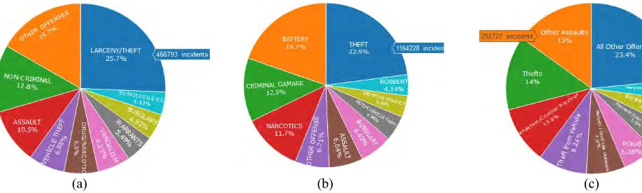
FIGURE 3. Top-10 crime cases for cities of (a) San-Francisco, (b) Chicago, and (c) Philadelphia.
percentages in Fig. 3. As seen, theft is a major problem that threatens each city, along with some violent crimes such as assaults and burglary.
The hourly trends unravel some interesting crime facts as shown in Fig. 4. As seen, crimes by hour in all three cities share similar patterns, where 5-6 am is the safest part of the day whilst 0 am is the most dangerous hour with the most crime incidents reported. Also, 12 pm is also very danger-ous during a day and in fact the hour where the maximum incidents reported under some crime categories. This actually is reasonable as it is the time when more people go out for lunch and also the time when tired criminals become aggres-sive under limited police available [43]. As a result, more police resources should be allocated in the shift from noon
to midnight if the police force is limited. We also noticed that Chicago has more crimes than the other two cities, and San Francisco is only one-third of the size of Philadelphia but has the same number of criminal cases. From American census data we know that Chicago has more population and larger area, which explains somehow more crimes it has. When calculating the population density as person/square mile, however, it becomes 17179 for San-Francisco, 11841 for Chicago, and 11379 for Philadelphia, this actually is another main factor that boosts crimes [44].
[image:4.576.48.507.384.522.2]FIGURE 4. Hourly trend of crime in each city.
[image:5.576.46.510.67.227.2]FIGURE 5. Wordcloud of crime description in each city: (a) San-Francisco, (b) Chicago, (c) Philadelphia.
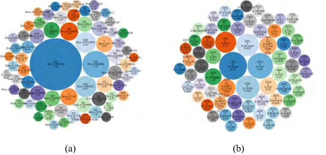
FIGURE 6. Bubble plot for street crime analysis: (a) San-Francisco, (b) Chicago, (c) Philadelphia.
related issues. Chicago, however, is plagued by domestic and battery crime as well as vehicle-related crimes. For Philadel-phia, the crime description is relatively simple, and the major problem of the city we discovered is related to theft, vehicle and assaults.
Fig. 6 shows the top streets where the maximum crime incidents were reported in the three cities. In San-Francisco the top three dangerous streets were Bryant Street, Market Street, and Mission Street. In Chicago these become Ohare Street, State Street, and Cicero Avenue. In Philadelphia,
Roosevelt BLVD, Frankford Avenue, and Market Street were the three streets with the most frequent crimes. These streets are all close to the downtown, where many financial districts, fortune 500 companies, and luxury hotels located nearby. This may be one reason that crime incidents boosts.
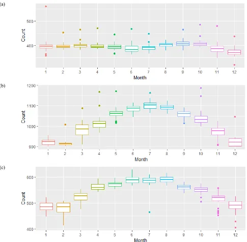
[image:5.576.43.369.412.567.2]FIGURE 7. Box plot of monthly statistics of crime in each city: (a) San-Francisco, (b) Chicago, (c) Philadelphia.
least safe month with the maximum number of reported crime incidents. For Philadelphia, the mean value of reported crimes in each day is 400-600 incidents with February the safest and June-August the least safe months. While Chicago has the most crimes reported among the three cities with a mean value of 1000 incidents per day, where February is the safest month followed by December and January. However, June-August are the most notorious months with the highest numbers of crime incidents.We found that monthly crime rate is very likely linked to local climates: With a Mediter-ranean climate, San-Francisco is warm hence people may share similar working and life patterns throughout the year.
Whilst Chicago and Philadelphia are temperate continental climate with a cold winter and hot summer in June- August, significant more outdoor living/activities can be found in summer than winter days thus the associated higher or lower crime incidents in different seasons.
IV. PREDICTION MODELS
FIGURE 8. Decomposed time series to show how crime evolved over time in three cities of San Francisco (a), Chicago (b), and Philadelphia (c). For each original time series (top), we show the estimated trend component (2ndtop), the estimated seasonal component (3rdtop), and the estimated irregular component (bottom).
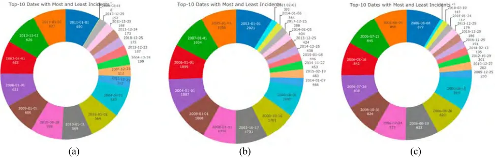
FIGURE 9. Top-10 dates with the most and least crimes: (a) San-Francisco, (b) Chicago, (c) Philadelphia.
successive data points within a time series are equally spaced in time, hence these data are discrete in time. Fig. 8 demon-strates how the amount of crime incidents changed over time, which clearly show the potential trend and seasonal-ity in the data as analyzed and discussed in the following sections.
A. PROPHET MODEL
The Prophet model is a procedure for forecasting time series data based on an additive model where non-linear trends are fit with yearly, weekly, and/or daily seasonality, plus holiday effects [36]. It works best with time series that have strong seasonal effects and cover several seasons of histor-ical data. The Prophet model is robust to missing data and shifts in the trend, and typically it handles outliers well. The Prophet model is designed to handle complex features in time series, it also designed to have intuitive parameters that can be adjusted without knowing the details of the underlying model.
The Prophet model decomposes time series into three main components, i.e. the trend, seasonality, and holidays. They are combined in the following equation:
y(t) = g(t) + s(t) + h(t) +εt (1)
where g(t) is the trend of any non-periodic changes in the time series, s(t) represents periodic changes (e.g., weekly and yearly seasonality), and h(t) represents the holiday effects of any potentially irregular schedules over one or more days. The error termεt represents any random effects which are not accommodated by the model.
For the trend function g(t), we utilized a linear trend with limited change points, where a piece-wise constant rate of growth provides a parsimonious and useful model.
g(t)=(k+a(t)Tδ)t+(m+a(t)Tγ) (2)
aj(t)=
(
1, if t ≥sj,
0, otherwise. (3)
where k is the growth rate,δis the rate adjustment, m is the offset parameter, andγ is set to−sjδjto make the function continuous.
Crime data is time series with multi-period seasonality, e.g. daily, weekly and annually. To this end, the seasonal function relies on Fourier series defined below, where P denotes the regular period:
s(t)= N
X
n=1
(ancos(2πnt
P )+bnsin( 2πnt
[image:7.576.46.533.256.413.2]As for holidays related events, they are defined by gener-ating a matrix of regressors:
Z(t)=[l(t ∈D1, . . . ,l(t ∈DL))] (5)
h(t)=Z(t)k (6)
where Di is the set of past and future dates for holidays, k ∼ Normal(0,ν2), l is an indicator function representing whether time t is during holiday i, Z(t) is the regressor matrix.
B. NEURAL NETWORK MODEL
A neural network is composed of a certain numbers of neu-rons, namely nodes in the network, which are organized in several layers and connected to each other cross different layers [45]. There are at least three layers in a neural network, i.e. the input layer of the observations, a non-observable hidden layer in the middle, and an output layer as the pre-dicted results. In this paper we explored the multilayer feed-forward network, where each layer of nodes receives inputs from the previous layer. The outputs of the nodes in one layer will become the inputs to the next layer. The inputs to each node are combined using a weighted linear combination below [46]:
zj=bj+ n
X
i=1
ωi,jxi (7)
The hidden layer will modify the input above using a nonlinear function by
s(z)= 1
1+e−z (8)
C. LSTM MODEL
LSTM model is a powerful type of recurrent neural network (RNN), capable of learning long-term dependencies [47]. For time series involves auto-correlation, i.e. the presence of correlation between the time series and lagged versions of itself, LSTMs are particular useful in prediction due to their capability of maintaining the state whilst recognizing pat-terns over the time series. The recurrent architecture enables the states to be persisted, or communicate between updated weights as each epoch progresses. Moreover, the LSTM cell architecture can enhance the RNN by enabling long term persistence in addition to short term [48].
f(t)=σ(Wf · [ht−1,xt]+bf) (9)
it =σ(Wi· [ht−1,xt]+bi) (10)
∼
C t
=tanh(WC· [ht−1,xt]+bC) (11)
Ct =ft∗Ct−1+it∗
∼
C
t (12)
where, ftis a sigmoid function to indicate whether to keep the previous state, Ct−1is the old cell state, Ctis the updated cell state, Wf, Wi, and WCare the previous value in each layer, ht−1and xt,is the input value, bf, bi,and bcare constant values, it decides which value will be used to update the state, Ct stands for the new candidate values.
V. EXPRRIMENTAL RESULTS
A. DECOMPOSE OF TIME SERIES
Time series can exhibit a variety of patterns, and it is always helpful to decompose a time series into several components, each representing an underlying pattern category. Fig. 8 illus-trates a decomposed crime time series, where for each orig-inal time series on the top, the three decomposed parts can respectively show the estimated trend component, seasonal component, and irregular component, respectively. The esti-mated trend component has shown that the overall crimes in San-Francisco slightly decreased from 2003 to 2013, fol-lowed by a steady increase from then on to 2017. However, crimes in Chicago seemed to decrease quickly from 2003 to 2015 and then became quite stable, whilst in Philadelphia the number of crimes had a downward trend yet with some undulations until it became stable after 2016. Regarding the seasonal component, it changes slowly over the time, where a quite strong annual periodic pattern can be observed for Chicago and Philadelphia than San-Francisco. This may be due to the more apparent annual climate changes in the two cities, where the crimes reached the peak in the middle of the year when the temperature becomes the hottest. As such, time series models will perform well on these datasets to forecast crimes in the future.
B. RESULTS ANALYSIS
We have explored deep learning algorithms and time series forecast models to predict crime trends. For performance evaluation, the Root Mean Square Error (RMSE) and spear-man correlation [49] are used in terms of different parameters and different sizes of training samples. The RMSE and spear-man correlation are defined as follows.
RMSE = v u u t 1 n n X
i=1 (Yi−
∼
Yi)2 (13)
ρX,Y =
cov(X,Y) σXσY
(14)
where Yi and Y are the true values;
∼
Yi and X are predicted values; cov is the covariance;σXis the standard deviation of X, andσY is the standard deviation of Y.
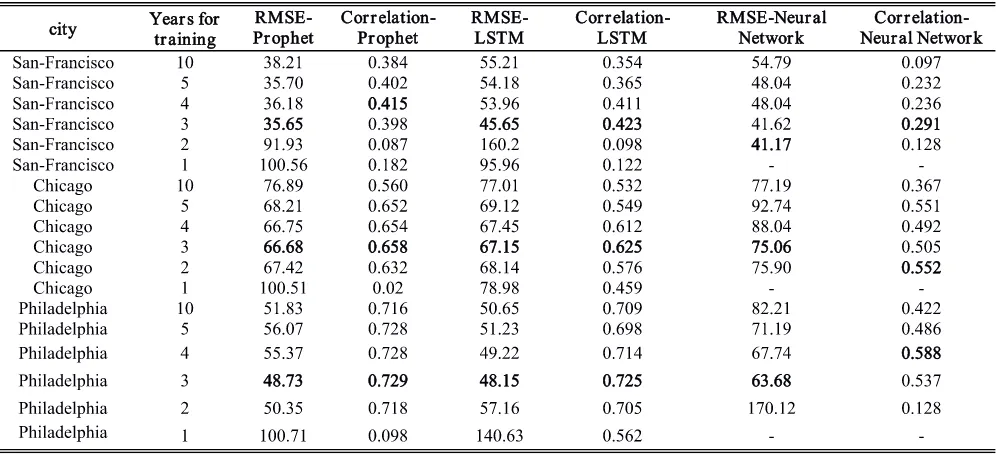
TABLE 1. Comparison of different algorithms/models in terms of RMSE and spearman correlation under different sizes of training samples.
TABLE 2. Comparison of different changepoint ranges in the prophet model in terms of RMSE and spearman correlation.
FIGURE 10. Crime trends in 2018 using prophet model with 3 years training data in (a) San-Francisco, (b) Chicago, (c) Philadelphia.
The results also showed that Prophet model and LSTM model performed better than traditional neural network models as demonstrated in table. 1 that neural network seems has lower RMSE but the correlation between predicted values and the real ones is low. The visualization of the trends in Fig. 10, 11, and 12 also conforms this conclusion.
[image:9.576.44.531.502.617.2]FIGURE 11. Crime trends in 2018 using state LSTM model with 3 years training data in (a) San-Francisco, (b) Chicago, (c) Philadelphia.
FIGURE 12. Crime trends in 2018 using neural network model with 3 years training data in (a) San-Francisco, (b) Chicago, (c) Philadelphia.
TABLE 3. Comparison of different layers in the LSTM model in terms of RMSE and spearman correlation.
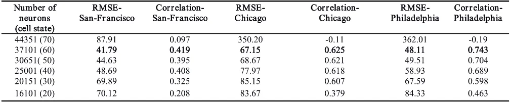
TABLE 4. Comparison of different number of neuros (cell state) in the LSTM model in terms of RMSE and spearman correlation.
incidents respectively, thus we set these 20 dates as holidays. Moreover, we analyzed different changepoint ranges, refer-ring to the proportion of history in which trend changepoints will be estimated. According to the results shown in Table 2, the best changepoint range is determined as 0.8, which means that the first 80 points are specified as changepoints. For the LSTM model, we first investigated the effect of
[image:10.576.36.538.389.490.2] [image:10.576.35.540.525.626.2]is computed as 50. The number of neurons in our model is affected largely by a parameter called cell state, we found that when the cell state is set as 60, we get the optimal results.
With the derived best training period as three years and the optimal parameters for the Prophet and the LSTM models, we predict the crimes for the three cities in 2018 as shown in Fig. 9, Fig. 10 and Fig. 11 respectively. All predictive results indicate that crime in 2018 may decrease but still boost in some months. When compared with part of the data available in 2018, our results show relatively low RMSE and high correlation with the new data. As such we suggest that police department deploy more forces in summer and citizens be more cautious when going out.
VI. CONCLUSION & FUTURE WORK
In this paper a series of state-of-the-art big data analytics and visualization techniques were utilized to analyze crime big data from three US cities, which allowed us to identify patterns and obtain trends. By exploring the Prophet model, a neural network model, and the deep learning algorithm LSTM, we found that both the Prophet model and the LSTM algorithm perform better than conventional neural network models. We also found the optimal time period for the training sample to be 3 years, in order to achieve the best prediction of trends in terms of RMSE and spearman correlation. Optimal parameters for the Prophet and the LSTM models are also determined. Additional results explained earlier will provide new insights into crime trends and will assist both police departments and law enforcement agencies in their decision making.
In future, we plan to complete our on-going platform for generic big data analytics which will be capable of processing various types of data for a wide range of applications. We also plan to incorporate multivariate visualization [59], graph min-ing techniques [54] and fine-grained spatial analysis [60] to uncover more potential patterns and trends within these datasets. Moreover, we aim to conduct more realistic case studies to further evaluate the effectiveness and scalability of the different models in our system.
REFERENCES
[1] A. Gandomi and M. Haider, ‘‘Beyond the hype: Big data concepts, meth-ods, and analytics,’’Int. J. Inf. Manage., vol. 35, no. 2, pp. 137–144, Apr. 2015.
[2] J. Zakir and T. Seymour, ‘‘Big data analytics,’’Issues Inf. Syst., vol. 16, no. 2, pp. 81–90, 2015.
[3] Y. Wang, L. Kung, W. Y. C. Wang, and C. G. Cegielski, ‘‘An integrated big data analytics-enabled transformation model: Application to health care,’’ Inf. Manage., vol. 55, no. 1, pp. 64–79, Jan. 2018.
[4] U. Thongsatapornwatana, ‘‘A survey of data mining techniques for ana-lyzing crime patterns,’’ in Proc. 2nd Asian Conf. Defence Technol., Chiang Mai, Thailand, 2016, pp. 123–128.
[5] W. Raghupathi and V. Raghupathi, ‘‘Big data analytics in healthcare: Promise and potential,’’Health Inf. Sci. Syst., vol. 2, no. 1, pp. 1–10, Feb. 2014.
[6] J. Archenaa and E. A. M. Anita, ‘‘A survey of big data analytics in healthcare and government,’’Procedia Comput. Sci., vol. 50, pp. 408–413, Apr. 2015.
[7] A. Londhe and P. Rao, ‘‘Platforms for big data analytics: Trend towards hybrid era,’’ inProc. Int. Conf. Energy, Commun., Data Anal. Soft Comput. (ICECDS), Chennai, 2017, pp. 3235–3238.
[8] W. Grady, H. Parker, and A. Payne, ‘‘Agile big data analytics: AnalyticsOps for data science,’’ inProc. IEEE Int. Conf. Big Data, Boston, MA, USA, Dec. 2017, pp. 2331–2339.
[9] R. Vatrapu, R. R. Mukkamala, A. Hussain, and B. Flesch, ‘‘Social set analysis: A set theoretical approach to Big Data analytics,’’IEEE Access, vol. 4, pp. 2542–2571, 2016.
[10] Y. Zhang, S. Ren, Y. Liu, and S. Si, ‘‘A big data analytics architecture for cleaner manufacturing and maintenance processes of complex products,’’ J. Cleaner Prod., vol. 142, no. 2, pp. 626–641, Jan. 2017.
[11] E. W. Ngai, A. Gunasekaran, S. F. Wamba, S. Akter, and R. Dubey, ‘‘Big data analytics in electronic markets,’’Electron. Markets, vol. 27, no. 3, pp. 243–245, Aug. 2017.
[12] Y.-Y. Liu, F.-M. Tseng, and Y.-H. Tseng, ‘‘Big Data analytics for fore-casting tourism destination arrivals with the applied Vector Autoregres-sion model,’’Technol. Forecasting Social Change, vol. 130, pp. 123–134, May 2018.
[13] D. Fisher, M. Czerwinski, S. Drucker, and R. DeLine, ‘‘Interactions with big data analytics,’’Interactions, vol. 19, no. 3, pp. 50–59, Jun. 2012. [14] C.-H. Yu, M. Morabito, P. Chen, and W. Ding, ‘‘Hierarchical
spatio-temporal pattern discovery and predictive modeling,’’IEEE Trans. Knowl. Data Eng., vol. 28, no. 4, pp. 979–993, Apr. 2016.
[15] S. Musa, ‘‘Smart cities—A road map for development,’’IEEE Potentials, vol. 37, no. 2, pp. 19–23, Mar./Apr. 2018.
[16] S. Wang, X. Wang, P. Ye, Y. Yuan, S. Liu, and F.-Y. Wang, ‘‘Parallel crime scene analysis based on ACP approach,’’IEEE Trans. Computat. Social Syst., vol. 5, no. 1, pp. 244–255, Mar. 2018.
[17] S. Yadav, A. Yadav, R. Vishwakarma, N. Yadav, and M. Timbadia, ‘‘Crime pattern detection, analysis & prediction,’’ in Proc. IEEE Int. Conf. Electron., Commun. Aerosp. Technol., Coimbatore, India, Apr. 2017, pp. 225–230.
[18] N. Baloian, C. E. Bassaletti, M. Fernández, O. Figueroa, P. Fuentes, R. Manasevich, M. Orchard, S. Peñafiel, J. A. Pino, and M. Vergara, ‘‘Crime prediction using patterns and context,’’ in Proc. 21st IEEE Int. Conf. Comput. Supported Cooperat. Work Design, Wellington, New Zealand, Apr. 2017, pp. 2–9.
[19] X. Zhao and J. Tang, ‘‘Exploring transfer learning for crime prediction,’’ inProc. IEEE Int. Conf. Data Mining Workshops, New Orleans, LA, USA, Nov. 2017, pp. 1158–1159.
[20] S. Wu, J. Male, and E. Dragut, ‘‘Spatial-temporal campus crime pattern mining from historical alert messages,’’ inProc. Int. Conf. Comput., Netw. Commun., Santa Clara, CA, USA, 2017, pp. 778–782.
[21] K. R. S. Vineeth, T. Pradhan, and A. Pandey, ‘‘A novel approach for intelligent crime pattern discovery and prediction,’’ inProc. Int. Conf. Adv. Commun. Control Comput. Technol., Ramanathapuram, India, 2016, pp. 531–538.
[22] C. R. Rodríguez, D. M. Gomez, and M. A. M. Rey, ‘‘Forecasting time series from clustering by a memetic differential fuzzy approach: An application to crime prediction,’’ inProc. IEEE Symp. Ser. Comput. Intell., Honolulu, HI, USA, Nov./Dec. 2017, pp. 1–8.
[23] A. Joshi, A. S. Sabitha, and T. Choudhury, ‘‘Crime analysis using K-means clustering,’’ inProc. 3rd Int. Conf. Comput. Intell. Netw., Odisha, India, 2017, pp. 33–39.
[24] N. M. M. Noor, W. M. F. W. Nawawi, and A. F. Ghazali, ‘‘Supporting decision making in situational crime prevention using fuzzy association rule,’’ inProc. Int. Conf. Comput., Control, Informat. Appl. (IC3INA), Jakarta, Indonesia, 2013, pp. 225–229.
[25] M. Wang, F. Zhang, H. Guan, X. Li, G. Chen, T. Li, and X. Xi, ‘‘Hybrid neural network mixed with random forests and Perlin noise,’’ inProc. 2nd IEEE Int. Conf. Comput. Commun. (ICCC), Chengdu, China, Oct. 2016, pp. 1937–1941.
[26] Z. Wang, D. Zhang, M. Sun, J. Jiang, and J. Ren, ‘‘A deep-learning based feature hybrid framework for spatiotemporal saliency detection inside videos,’’Neurocomputing, vol. 287, pp. 68–83, Apr. 2018.
[27] J. Ren and J. Jiang, ‘‘Hierarchical modeling and adaptive clustering for real-time summarization of rush videos,’’IEEE Trans. Multimedia, vol. 11, no. 5, pp. 906–917, Aug. 2009.
[28] J. Han, G. Cheng, L. Guo, J. Ren, and D. Zhang, ‘‘Object detection in optical remote sensing images based on weakly supervised learning and high-level feature learning,’’IEEE Trans. Geosci. Remote Sens., vol. 53, no. 6, pp. 3325–3337, Jun. 2014.
[30] Y. Yan, J. Ren, G. Sun, H. Zhao, J. Han, X. Li, S. Marshall, and J. Zhan, ‘‘Unsupervised image saliency detection with gestalt-laws guided opti-mization and visual attention based refinement,’’Pattern Recognit., vol. 79, pp. 65–78, Jul. 2018.
[31] Z. Zhao, S. Tu, J. Shi, and R. Rao, ‘‘Time-weighted LSTM model with redefined labeling for stock trend prediction,’’ inProc. IEEE 29th Int. Conf. Tools Artif. Intell. (ICTAI), Boston, MA, USA, Nov. 2017, pp. 1210–1217. [32] J. Dai, G. Sheng, X. Jiang, and H. Song, ‘‘LSTM networks for the trend prediction of gases dissolved in power transformer insulation oil,’’ inProc. 12th Int. Conf. Properties Appl. Dielectr. Mater., Xi’an, China, 2018, pp. 666–669.
[33] H. Kashef, M. Abdel-Nasser, and K. Mahmoud, ‘‘Power loss estimation in smart grids using a neural network model,’’ inProc. Int. Conf. Innov. Trends Comput. Eng. (ITCE), Aswan, Egypt, 2018, pp. 258–263. [34] H. Hassani, X. Huang, M. Ghodsi, and E. S. Silva, ‘‘A review of data
mining applications in crime,’’Stat. Anal. Data Mining, ASA Data Sci. J., vol. 9, no. 3, pp. 139–154, Apr. 2016.
[35] Z. Jia, C. Shen, Y. Chen, T. Yu, X. Guan, and X. Yi, ‘‘Big-data analysis of multi-source logs for anomaly detection on network-based system,’’ in Proc. 13th IEEE Conf. Autom. Sci. Eng. (CASE), Xi’an, China, Aug. 2017, pp. 1136–1141.
[36] A. Agresti,An Introduction to Categorical Data Analysis, 3rd ed. Hoboken, NJ, USA: Wiley, 2018.
[37] M. Huda, A. Maseleno, M. Siregar, R. Ahmad, K. A. Jasmi, N. H. N. Muhamad, and P. Atmotiyoso, ‘‘Big data emerging technology: Insights into innovative environment for online learning resources,’’Int. J. Emerg. Technol. Learn., vol. 13, no. 1, pp. 23–36, Jan. 2018. [38] San Francisco Crime Data. [Online]. Available: https://data.sfgov.org/
Public-Safety/Police-Department-Incident-Reports-Historical-2003/tmnf-yvry
[39] Chicago Crime Data. [Online]. Available: https://data.cityofchicago. org/Public-Safety/Crimes-2001-to-present/ijzp-q8t2
[40] Philadelphia Crime Data. [Online]. Available: https://www. opendataphilly.org/dataset/crime-incidents
[41] V. Viswanathan and S. R. Viswanathan,Data Analysis Cookbook, 2nd ed. Birmingham, U.K.: Packt Publishing Ltd, 2015, pp. 30–39.
[42] R. Boix, B. De Miguel-Molina, and J. L. Hervás-Oliver, ‘‘Micro-geographies of creative industries clusters in Europe: From hot spots to assemblages,’’Papers Regional Sci., vol. 94, no. 4, pp. 753–772, Jan. 2015. [43] Z. Krizan and A. D. Herlache, ‘‘Sleep disruption and aggression: Impli-cations for violence and its prevention,’’Psychol. Violence, vol. 6, no. 4, pp. 542–552, Oct. 2016.
[44] US Population Density by City. [Online]. Available: http://www.governing. com/blogs/by-the-numbers/most-densely-populated-cities-data-map.html [45] I. N. da Silva and D. H. Spatti, ‘‘Introduction,’’ inArtificial Neural
Net-works. Cham, Switzerland: Springer, 2017, pp. 3–19.
[46] R. J. Hyndman and G. Athanasopoulos,Forecasting: Principles and Prac-tice, 2nd ed. OTexts, 2018, pp. 333–339.
[47] K. Greff, R. K. Srivastava, J. Koutnìk, B. R. Steunebrink, and J. Schmidhuber, ‘‘LSTM: A search space odyssey,’’IEEE Trans. Neural Netw. Learn. Syst., vol. 28, no. 10, pp. 2222–2232, Oct. 2017.
[48] J. Lai, B. Chen, S. Tong, K. Yu, and T. Tan, ‘‘Phone-aware LSTM-RNN for voice conversion,’’ inProc. IEEE 13th Int. Conf. Signal Process. (ICSP), Chengdu, China, Nov. 2016, pp. 177–182.
[49] P. Schober, C. Boer, and L. A. Schwarte, ‘‘Correlation coefficients: Appro-priate use and interpretation,’’ Anesthesia Analgesia, vol. 126, no. 5, pp. 1763–1768, May 2018.
[50] American Cities With the Worst Income Inequality. [Online]. Avail-able: https://www.cbsnews.com/media/9-american-cities-with-the-worst-income-inequality/
[51] M. Lofstrom and S. Raphael, ‘‘Crime, the Criminal Justice System, and Socioeconomic Inequality,’’J. Econ. Perspect., vol. 30, no. 2, pp. 26–103, Mar. 2016.
[52] L. Zhou, J. Wang, A. V. Vasilakos, and S. Pan, ‘‘Machine learning on big data: Opportunities and challenges,’’Neurocomputing, vol. 237, pp. 350–361, May 2017.
[53] M. Injadat, F. Salo, and A. B. Nassif, ‘‘Data mining techniques in social media: A survey,’’Neurocomputing, vol. 214, pp. 654–670, Nov. 2016. [54] Y. Gao, Y. Xia, J. Qiao, and S. Wu, ‘‘Solution to gang crime based on
graph theory and analytical hierarchy process,’’Neurocomputing, vol. 140, pp. 121–127, Sep. 2014.
[55] S. Zheng, S. Chen, L. Yang, J. Zhu, Z. Luo, J. Hu, and X. Yang, ‘‘Big data processing architecture for radio signals empowered by deep learning: Concept, experiment, applications and challenges,’’IEEE Access, vol. 6, pp. 55907–55922, 2018.
[56] J. Zhao, Y. Gao, Y. Qu, H. Yin, Y. Liu, and H. Sun, ‘‘Travel time prediction: Based on gated recurrent unit method and data fusion,’’IEEE Access, vol. 6, pp. 70463–70472, 2018.
[57] K. Niu, H. Zhang, C. Cheng, C. Wang, and T. Zhou, ‘‘A novel spatio-temporal model for city-scale traffic speed prediction,’’ IEEE Access, vol. 7, pp. 30050–30057, 2019.
[58] J. Peral, A. Ferrández, D. Gil, E. Kauffmann, and H. Mora, ‘‘A review of the analytics techniques for an efficient management of online forums: An architecture proposal,’’IEEE Access, vol. 7, pp. 12220–12240, 2019. [59] L. Stopar, P. Skraba, D. Mladenic, and M. Grobelnik, ‘‘StreamStory:
Exploring multivariate time series on multiple scales,’’IEEE Trans. Vis. Comput. Graphics, vol. 25, no. 4, pp. 1788–1802, Apr. 2019.
[60] L. Guo, X. Cai, F. Hao, D. Mu, C. Fang, and L. Yang, ‘‘Exploiting fine-grained co-authorship for personalized citation recommendation,’’IEEE Access, vol. 5, pp. 12714–12725, 2017.
MINGCHEN FENGreceived the M.S. degree in software engineering from the School of Software and Microelectronics, Northwestern Polytechni-cal University, Xi’an, China, in 2015, where he is currently pursuing the Ph.D. degree with the School of Computer Science. He was a Visiting Researcher with the Department of Electronic and Electrical Engineering, University of Strathclyde, Glasgow, U.K., in 2018. His research interests include big data analytics, data mining, machine learning, deep learning, and data visualization.
JIANGBIN ZHENGreceived the B.S., M.S., and Ph.D. degrees in computer science from North-western Polytechnical University, in 1993, 1996, and 2002, respectively.
From 2000 to 2002, he was a Research Assis-tant with The Hong Kong Polytechnic University, Hong Kong. From 2004 to 2005, he was a Research Assistant with The University of Sydney, Sydney, Australia. Since 2009, he has been a Professor and Ph.D. Supervisor with the School of Com-puter Science, Northwestern Polytechnical University. His research interests include intelligent information processing, visual computing, multimedia signal processing, big data, and soft engineering. He has published over 100 peer-reviewed journal/conference papers covering a wide range of topics in image/video analytics, pattern recognition, machine learning, and big data analytics.
JINCHANG REN received the B.E. degree in computer software, the M.Eng. degree in image processing, and the D.Eng. degree in computer vision from Northwestern Polytechnical Univer-sity, Xi’an, China. He received the Ph.D. degree in electronic imaging and media communication from Bradford University, Bradford, U.K.
AMIR HUSSAINreceived the B.Eng. (Hons.) and Ph.D. degrees from the University of Strathclyde, Glasgow, U.K., in 1992 and 1997, respectively. Following postdoctoral and academic positions held at the West of Scotland, from 1996 to 1998, Dundee, from 1998 to 2000, and Stirling Uni-versities, from 2000 to 2018, respectively. He is currently a Professor and the founding Head of the Cognitive Big Data and Cybersecurity (CogBiD) Research Lab with Edinburgh Napier University, U.K. He has coauthored more than 350 papers, including over a dozen books and around 140 journal papers. Amongst other distinguished roles, he is the General Chair for the IEEE WCCI 2020 (the world’s largest technical event in Computational Intelligence), and the Vice-Chair of the Emergent Technologies Technical Committee of the IEEE Computational Intelligence Society. He is also founding Editor-in-Chief of two leading journals: Cog-nitive Computation(Springer Nature), BMC Big Data Analytics (BioMed Central), of the Springer Book Series on Socio-Affective Computing, and Cognitive Computation Trends. He is also an Associate Editor for a number of prestigious journals, including:Information Fusion(Elsevier),AI Review (Springer), the IEEE TRANSACTIONS ON NEURAL NETWORKS AND LEARNING SYSTEMS, the IEEE Computational Intelligence Magazine, and the IEEE TRANSACTIONS ONEMERGINGTOPICS INCOMPUTATIONALINTELLIGENCE. He has led major national, EU and internationally funded projects and supervised over 30 Ph.D. students.
XIUXIU LI received the Ph.D. degree with the School of Computer Science, Northwestern Poly-technical University, Xi’an, China, in 2012. She is currently a Lecturer with the Xi’an University of Technology. Her research interests include com-puter vision and pattern recognition.
YUE XIreceived the B.S. degree from the Qingdao University of Technology, China, in 2011, the M.S. degree from Guizhou University, China, in 2014. He is currently pursuing the dual Ph.D. degrees in computer science with the University of Tech-nology Sydney, Australia, and Northwestern Poly-technical University, Xi’an, China. His research interests include computer vision, image process-ing, machine learnprocess-ing, and deep learning.