Implementation of peridynamic beam and plate formulations in finite element framework

O R I G I NA L A RT I C L E

Zhenghao Yang · Erkan Oterkus · Cong Tien Nguyen · Selda Oterkus

Implementation of peridynamic beam and plate formulations

in finite element framework

Received: 19 December 2017 / Accepted: 24 May 2018 © The Author(s) 2018

Abstract Peridynamic (PD) theory is a new continuum mechanics formulation introduced to overcome the limitations of classical continuum mechanics such as predicting crack initiation and propagation, and capturing nonlocal effects. PD theory is based on integro-differential equations and these equations are generally difficult to be solved by using analytical techniques. Therefore, numerical approximations, especially with meshless method, have been widely used. Numerical solution of three-dimensional models is usually computationally expensive and structural idealization can be utilized to reduce the computational time significantly. In this study, two of such structural idealization types are considered, namely Timoshenko beam and Mindlin plate, and their peridynamic formulations are briefly explained. Moreover, the implementation of these formulations in finite element framework is presented. To demonstrate the capability of the present approach, several case studies are considered including beam and plate bending due to transverse loading, buckling analysis and propagation of an initial crack in a plate under bending loading.

Keywords Peridynamics·Beam·Plate·Fracture·Finite element

1 Introduction

Peridynamic (PD) theory was introduced by Silling [33] to overcome limitations of Cauchy’s classical contin-uum mechanics (CCM) formulation for certain problems and conditions such as predicting crack initiation and propagation, and capturing nonlocal effects. PD theory is basically a new formulation of continuum mechan-ics. As opposed to partial differential equations of CCM, PD theory is based on integro-differential equations without having any spatial derivatives. Therefore, these equations are always valid regardless of displace-ment discontinuities due to cracks, etc. The derivation of peridynamic equations using Lagrange’s equation is presented in Madenci and Oterkus [22]. Moreover, PD theory has an internal length scale parameter called horizon. By using horizon, it may be possible to capture nonlocal effects which can appear in various problems especially at small scales. As argued by dell’Isola et al. [5–8], the origins of PD go back to Piola’s continuum formulation. Since its introduction in 2000, PD theory has been applied to many different material systems [12,18,27] and extended to other fields for heat transfer analysis, diffusion, etc. [10,16,28,29]. Queiruga and Moridis [32] performed numerical experiments on the convergence properties of state-based peridynamic laws and influence functions in two-dimensional problems.

It is difficult to solve integro-differential equations of peridynamics by using analytical techniques although analytical solutions for some simplified cases are available [24]. Instead numerical approaches are widely used

Communicated by Francesco dell’Isola. Z. Yang·E. Oterkus (

B

mainly utilizing meshless discretization concept [34]. Meshless approaches are especially useful for analyzing large deformations. In PD theory, each material point has a domain of influence, i.e., horizon and the material point interacts with all other material points inside its horizon. Therefore, as opposed to the nearest neighbor interaction assumption of CCM, points which are far from each other can also interact in a nonlocal fashion. Moreover, in PD theory, each point has three translational degrees of freedom for three-dimensional models. To obtain the displacements of each point, three equations of motion in x-, y- andz-directions in the form of integro-differential equations should be solved. Static solution can be obtained either by using adaptive dynamic relaxation (ADR) technique [19] or solving a system of equations. For dynamic solution, after obtaining acceleration of a point from the equation of motion at particular time, implicit or explicit time integration schemes can be used to determine the new location and velocity of the point at the next time step [22].

Numerical solution of PD equations is very suitable to be done in a parallel programming environment. The solution domain can be split into multiple parts and each part can be solved by a different processor which can decrease the computational time significantly. However, even with the current high performance computing capabilities, solution of three-dimensional problems with large number of degrees of freedom and small-time step sizes can still be challenging. To overcome this problem, structural idealizations such as beam and plate formulations can be utilized. Such formulations are available in PD theory framework. For instance, Diyaroglu et al. [13] proposed an ordinary state-based Euler beam formulation to be used for slender beam structures. Taylor and Steigmann [36] developed a peridynamic plate model based on bond-based formulation by using an asymptotic analysis for thin plates. Moreover, O’Grady and Foster [25,26] developed a non-ordinary state-based peridynamic model for Euler–Bernoulli beam and Kirchhoff–Love plate formulations by disregarding the transverse shear deformations. For thick beams and plates, Diyaroglu et al. [11] introduced peridynamic Timoshenko beam and Mindlin plate formulations considering transverse shear deformations, which will also be the foundation of the current study.

Computer implementation of peridynamic formulations is usually done by using a particular programming language such as Fortran, C++. Although this approach is useful for research purposes, the applicability of these codes in a wider public may be limited since many researchers and engineers are using commercial software with user-friendly graphical user interfaces, efficient solution algorithms, etc. Therefore, in this study, the implementation of peridynamic beam and plate formulations in a commercial finite element (FE) software will be presented. Several benchmark problems are considered to demonstrate the accuracy and practicality of the current approach. Peridynamic solutions are compared against regular FE solutions [2] due to its simplicity and accuracy for problems without discontinuity [1,3,14].

2 Peridynamic Timoshenko beam and mindlin plate formulation

PD theory is based on the same continuum assumption as in CCM. According to this assumption, the body is composed of infinitely small volumes called material points. In the undeformed state of the body, each material point is identified by its coordinates, x₍k) with(k = 1,2, . . . ,∞), and is associated with an incremental volume,V₍k), and a mass density ofρ(x(k)). In this section, peridynamic Timoshenko beam and Mindlin plate formulations will be briefly presented based on the study by Diyaroglu et al. [11].

2.1 Peridynamic Timoshenko beam formulation

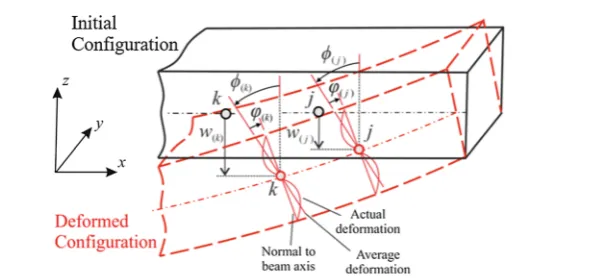
For the material pointkin a Timoshenko beam shown in Fig.1, the peridynamic interaction forces between material points j andkarising from transverse shear deformation, fˆ₍k)(j)and bending, f˜(k)(j) can be defined for a linear material behavior as

ˆ

f₍k)(j) =csϕ(k)(j) (1) and

˜

Fig. 1 Initial and deformed configurations of a Timoshenko beam

arising from the interaction between material points j andkcan be defined as the average of the transverse shear angles at these material points in the form

ϕ(k)(j)=

w(j)−w(k)

ξ(j)(k) −

φ(j)+φ(k)

2 sgn

x₍j)−x(k)

(3)

where w andφ represent the out-of-plane deflection and rotation of sections, respectively, sgn(·)function provides the sign of the associated function, andξ₍j)(k)represents the initial distance between material points

j andk.

The curvature,κ₍k)(j), between the material points jandkcan be expressed as

κ(k)(j)=

φ(j)−φ(k)

ξ(j)(k)

(4)

Utilizing the definitions given in Eqs. (1–4), the peridynamic equations of motion for a Timoshenko beam can be obtained as

ρw¨(k)=cs ∞

j=1 _w

(j)−w(k)

ξ(j)(k) −

φ(j)+φ(k)

2 sgn

x₍j)−x(k)

V₍j)+ ˆb(k) (5a)

and

ρI

A φ¨(k)=cb

∞

j=1

φ(j)−φ(k)

ξ(j)(k)

V₍j)

+1

2cs ∞

j₌1 _w

(j)−w(k)

ξ(j)(k)

sgnx₍j)−x(k)

−φ(j)+φ(k) 2

ξ(j)(k)V(j)+ ˜b(k) (5b)

wherebˆ₍k)andb˜(k)represent body load and body moment terms,ρ,I, andAdenote mass density, moment of inertia and cross-sectional area of the beam, respectively, andV₍j)is the volume of material point j.

If peridynamic interactions are limited within the horizon of a material point, then these equations can be written in integral form as

ρw (¨ x,t)=cs

H

wx,t−w (x,t)

ξ −

φx,t+φ (x,t)

2 sgn

x−x dV+ ˆb(x,t) (6a)

and

ρI

A φ (¨ x,t)=

H

cbφ

x,t−φ (x,t)

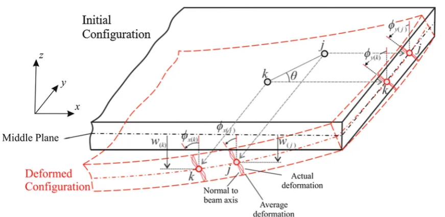
Fig. 2 Initial and deformed configurations of a Mindlin plate

+

H

1 2cs

wx,t−w (x,t)

ξ sgn

x−x−φ

x,t+φ (x,t)

2 ξ dV

_{+ ˜b(x,t)}

(6b)

The PD material constantscsandcbcan be expressed in terms of shear and Young’s moduli,GandE, as

cs= 2ksG

Aδ2 andcb=

2E I

δ2_A2 (7a,b)

whereksis the shear correction factor.

2.2 Peridynamic mindlin plate formulation

Considering the material pointkas the point of interest as shown in Fig.2, the transverse shear angle,ϕ₍k)(j), between material points j andkcan be defined as the average of the shear angles at these material points in the form

ϕ(k)(j)= w(

j₎−w₍k₎

ξ(j)(k) −

φ(j₎+φ₍k₎

2 (8)

whereφ₍j)andφ(k)represent the rotations with respect to the line of action between the material points jand

kand can be defined as

φ(j) =φx(j)cosθ+φy(j)sinθ (9a)

φ(k) =φx(k)cosθ+φy(k)sinθ (9b) withθ being the orientation of the bond with respect tox-axis,φx andφy are rotations aroundy- andx-axis, respectively.

As for the Timoshenko beam, the curvature,κ₍k)(j), with respect to the line of action between the material points j andkcan be defined as

κ(k₎₍j₎ = φ(

j₎−φ₍k₎

ξ(j)(k)

(10)

When considering the material point jas the point of interest, the transverse shear angle and curvature for the interaction between the material points jandkbecome

ϕ(j)(k)= w(

k)−w(j)

ξ(j)(k) −

−φ(k)+φ(j) 2

and

κ(j)(k) = φ(

k)−φ(j)

ξ(j)(k)

(11b)

By using the same peridynamic interaction forces between material points j andkgiven in Eqs. (1,2) for a Timoshenko beam and utilizing the definitions given in Eqs. (8–11), the peridynamic equations of motion for a Mindlin plate can be written as

ρhw¨₍k)=cs ∞

j=1 _w

(j)−w(k)

ξ(j)(k) −

φx(j)+φx(k)

2 cosθ−

φy(j)+φy(k)

2 sinθ

V₍j)+ ˆb(k) (12a)

ρh3

12φ¨x(k)=cb ∞

j=1

φx(j)−φx(k)

ξ(j)(k)

cosθ+

φy(j)−φy(k)

ξ(j)(k)

sinθ

cosθV₍j)

+1

2cs ∞

j=1 ξ(j)(k)

w(j₎−w₍k₎

ξ(j)(k) −

φx₍j₎+φx₍k₎

2 cosθ−

φy₍j₎+φy₍k₎

2 sinθ

cosθV₍j)+ ˜bx(k)

(12b)

and

ρh3

12φ¨y(k)=cb ∞

j=1 _φ

x(j)−φx(k)

ξ(j)(k)

cosθ+

_φ

y(j)−φy(k)

ξ(j)(k)

sinθ

sinθV₍j)

+1

2cs ∞

j₌1 ξ(j)(k)

_w

(j)−w(k)

ξ(j)(k) −

φx(j)+φx(k)

2 cosθ−

φy(j)+φy(k)

2 sinθ

sinθV₍j)+ ˜by(k)

(12c)

or they can be expressed in continuous form as

ρhw (¨ x,t)=cs

H

wx,t−w (x,t)

ξ −

φx

x,t+φx(x,t)

2 cosθ−

φy

x,t+φy(x,t)

2 sinθ

×dV+ ˆb(x,t) (12d)

ρh3

12φ¨x(x,t)=cb

H

φx

x,t−φx(x,t)

ξ cosθ+

φy

x,t−φy(x,t)

ξ sinθ

cosθdV

+1

2cs

H

ξ

wx,t−w (x,t)

ξ −

φxx,t+φx(x,t)

2 cosθ−

φyx,t+φy(x,t)

2 sinθ

×cosθdV+ ˜bx(x,t) (12e)

and

ρh3

12φ¨y(x,t)=cb

H

φx

x,t−φx(x,t)

ξ cosθ+

φy

x,t−φy(x,t)

ξ sinθ

sinθdV

+1

2cs

H

ξ

wx,t−w (x,t)

ξ −

φx

x,t+φx(x,t)

2 cosθ

−φy

x,t+φy(x,t)

2 sinθ sinθdV

_{+ ˜b}

Note that the peridynamic interactions can be restricted within the horizon of material points, H. Therefore, the PD material constantscsandcbcan be expressed in terms of Young’s modulus,E, as

cs= 9E

4πδ3k 2

s andcb= 3h2E

4πδ3 (13a,b)

wherehis the thickness of the plate and Poisson’s ratio is equal toν =1/3. The PD material parameterscb andcsare determined for a material point whose horizon is completely embedded in the material. For material points close to boundaries require correction and the details of the correction procedure are given in Diyaroglu et. al. [11].

In order to include failure in the material response, the response functions in the equations of motion for the beam and plate can be modified through a history-dependent scalar value function,H(x₍j)−x(k),t)as

ˆ

f₍k)(j)=H

x₍j)−x(k),t

csϕ(k)(j) (14a)

and

˜

f₍k)(j)=H

x₍j)−x(k),t

cbκ(k)(j) (14b)

which is defined as

Hx₍j)−x(k),t

= 1 0 if otherwise

_κ(k)(j)

x₍j)−x(k),t< κc and ϕ(k)(j)

x₍j)−x(k),t< ϕc (15)

where critical curvature and angle values can be expressed in terms of Mode-I and Mode-III critical energy release rates of the material,GI candGI I I c, as

κc=

4GI c

cbhδ4

andϕc =

4GI I I c

cshδ4 ,

respectively. (16a, b)

Please note that although it is possible to make connections to some of the existing approaches for fracture modeling [17,23,31,35], there are also certain differences between peridynamics and other existing techniques, especially the peridynamic bond concept and its breakage under certain conditions.

3 Implementation of peridynamic formulations in finite element framework

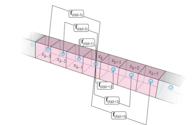
As mentioned earlier, analytical solution of peridynamic equations of motion is usually not possible and numerical approaches are widely utilized. If meshless method is used for spatial discretization, the solution domain is divided into finite number of volumes and each volume is represented by a point located at its center as shown in Fig.3. Each point is interacting with finite number of points located inside its horizon.

Peridynamic formulations can be numerically implemented using different computer languages in either serial or parallel manner. Moreover, commercial finite element softwares such as ANSYS, Abaqus can also be utilized by following the approach presented in Macek and Silling [21]. In this study, the implementation procedure of peridynamic Timoshenko beam and Mindlin plate formulations in a commercial finite element software will be presented.

3.1 Calibration process to link PD and classical FE parameters

As mentioned earlier, the unit of the peridynamic interaction force parameters between material points j and

k given in Eqs. (1) and (2) is force per volume squared. In order to convert these quantities to force, these expressions should be multiplied by the volumes of the associated material pointskand j as

˜

F₍k)(j) =cbκ(k)(j)V(k)V(j) (17a)

and

ˆ

Fig. 3 Meshless discretization of a domain and interaction between points inside the horizon of pointk

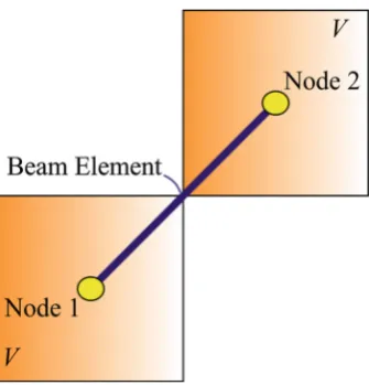
In finite element framework, each peridynamic interaction can be represented using a Timoshenko beam element. Corresponding forces for a Timoshenko beam element can be expressed as

˜

F₍k)(j) =E(k)(j)Iκ(k)(j) (18a)

and

ˆ

F₍k)(j)=G(k)(j)Aksϕ(k)(j) (18b)

in whichE₍k)(j) andG(k)(j)represent the Young’s modulus and shear modulus of the element, respectively, and I and Aare the moment of inertia and cross-sectional area. Equating the corresponding forces given in Eqs. (17) and (18) yields

E₍k)(j)=

cbV(k)V(j)

I (19a)

and

G₍k)(j) =

csV(k)V(j)

Aks

(19b)

Note that Young’s and shear moduli expressions given in Eqs. (19a,b) are not real material property values. Instead they are serving as the calibration parameters between peridynamics and finite element framework.

3.2 Implementation in ANSYS

Fig. 4 Beam element representing an interaction between PD points

Fig. 5 Network of beam elements to represent interactions between PD points

that BEAM188 has 6 degrees of freedom. Therefore, it can both represent bending behavior and in-plane (membrane) behavior. Hence, it can capture the effect of in-plane loading on bending deformations as in the buckling analysis.

3.3 Application of boundary conditions and loading

Peridynamic equations given in Eqs. (5) and (12) are obtained using Lagrange’s equations and without con-sidering the boundaries. Although there are currently different techniques available in the literature, in this study, the displacement and rotation boundary conditions are applied by introducing a fictitious layer with a thickness equivalent to the size of horizon [22]. Moreover, the loading is applied to a single layer of material points as a body load or moment.

4 Numerical results

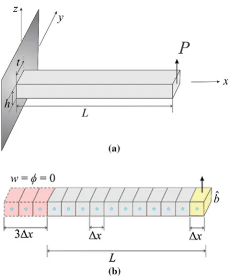
Fig. 6 aA cantilever beam subjected to transverse loading andbits discretization

can propagate in the current approach. The horizon size was chosen asδ=3.015xin all cases wherexis the uniform grid spacing.

4.1 Timoshenko beam

4.1.1 Beam bending

A cantilever beam shown in Fig.6with a length ofL=1 m and a cross-sectional area ofA=0.1×0.1 m2is considered. The Young’s modulus and Poisson’s ratio are specified asE =200GPa andν=1/3, respectively. The beam is discretized into a single row of material points with a distance between each other ofx=0.01 m. As suggested by Madenci and Oterkus [22], the left edge is constrained by introducing a fictitious region with a size of horizon,δ. Therefore, a total of 103 nodes are used in the model. A transverse concentrated force

P = −1000 N is applied to the right end of the beam.

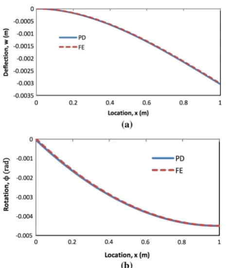
Figure7shows the deflection and rotation results obtained from both PD and classical FE models. It can be clearly seen that the solutions from PD model are in very good agreement with classical FE solution. This verifies the capability of PD Timoshenko beam formulation to capture small bending deformations and rotations.

4.1.2 Beam buckling

Same cantilever beam model considered in the previous case is tested for its buckling performance. When a structure is subjected to a compressive load, buckling may occur. The critical buckling load is the maximum load which a structure can resist buckling to occur.

Fig. 7 Variation ofadeflection andbrotation along the cantilever beam

Eigenvalue buckling analysis solution

According to Euler’s formula, the theoretical critical buckling load for the cantilever beam subjected to fixed-free end conditions can be calculated as

Fcr= π 2_{E I}

(2L)2 =4.11×10

6_{N (20)}

The same problem is also solved by using classical finite element method and peridynamic model performing an eigenvalue analysis. Both PD and classical FE solutions of critical buckling load from eigenvalue buckling analysis yield the same value of 4.08×106N which agree well with the theoretical value from Eq. (20). This clearly demonstrates that PD model of Timoshenko Beam has a good capability in eigenvalue analysis to predict critical buckling load.

No-linear buckling analysis solution

The performance of geometrical nonlinear buckling analysis of PD Timoshenko Beam is also studied. A total load of Fx = −5×106N is gradually applied to the beam at the right free end using 100 load steps. A sufficiently small transverse loading of Fy = −20,000 N(0.4% ofFx) is introduced to the free end to trigger the buckling behavior once the critical buckling load is reached.

In Fig.8, the variation of deflections as the load increases is demonstrated. The solutions of PD and classical FE agree very well with each other and both predicts that the beam becomes unstable and buckles at a load of approximately 4×106N, which is slightly less than the eigenvalue solution of 4.08×106N and theoretical value of 4.11×106N. Figure8also shows the post-buckling behavior of the column.

4.2 Plate

Fig. 8 Variation of deflection as the applied load increases

Fig. 9 aPlate subjected to transverse force loading andbits discretization

initial crack under bending loading is studied to demonstrate the failure prediction capability of the current formulation.

4.2.1 Bending

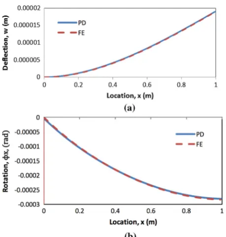
Fig. 10 Variation ofadeflection andbrotation along the centralx-axis of the plate.

horizon,δ. A transverse load is applied to a single row of material points as a body load at the right edge of the plate with an amount of 107N/m3.

As shown in Fig.10, the PD and classical FE solutions yield similar variation in terms of deflection and rotation for the points located along the centralx-axis. This shows that FE implementation of PD can accurately capture the bending behavior of the Mindlin plate.

4.2.2 Buckling

The cantilever plate considered in the previous case with same dimensions and material properties is also studied for its buckling behavior. As in the Timoshenko beam case, both eigenvalue and nonlinear buckling analysis are performed in this section.

Eigenvalue buckling analysis solution

The critical buckling load of the cantilever plate is first determined by performing an eigenvalue buckling analysis. Both PD and classical FE analyses yield same critical buckling load which is approximately equal to 4.35×105N.

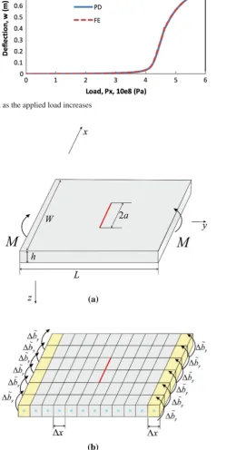
Nonlinear buckling analysis solutionThe performance of nonlinear buckling analysis of PD Mindlin plate is studied next. A total pressure of Px = −6×108N is gradually applied to the free edge of the plate, which is equivalent to a concentrated force of Fx = −6×105N, using 2000 load steps. To trigger the buckling behavior, a sufficiently small transverse load of Fy =2400 N (0.4% ofFx)is introduced to a single row of material points at the free edge.

In order to observe the buckling behavior of the plate, the deflection of the central point at free edge

(x = L,y= 0)is recorded as the load increases. As depicted in Fig.11, the PD and classical FE solutions are in very good agreement and both predicts that the plate buckles at a pressure loading of approximately 4.1×108Pa which is slightly less than the eigenvalue solution of 4.35×108Pa. Figure11also shows the post-buckling behavior of the cantilever plate.

4.2.3 Plate with an initial crack subjected to pure bending loading

Fig. 11 Variation of deflection as the applied load increases

Fig. 12 aA plate with a central crack subjected to pure bending loading andbits discretization

Fig. 13 Propagation of a central crack in a plate subjected to uniform bending loading

propagate when the resultant body load reachesb˜y = ±3.2×106N/m. This result is consistent with the result obtained by Diyaroglu et al. [11], and as expected, the crack propagates toward the edges of the plate as the load increases as shown in Fig.13.

5 Final remarks

The main purpose of this study is to present finite element implementation of peridynamic Timoshenko and Mindlin plate formulations. The advantage of this approach is that only one single row of material points along the thickness is required, which not only decreases the memory consumption by reducing the number of the nodes and elements, but also brings efficiency on processing speed. The feasibility and accuracy of the current approach is verified by considering various benchmark problems and comparing peridynamic results against classical finite element solutions in bending and buckling cases. A good agreement is obtained between peridynamic and finite element analyses results. Moreover, crack growth in a plate subjected to bending loading case is studied to demonstrate the failure prediction capability of the current approach. As a future study, impact analysis will be considered to extend the usage of the current approach. Developed framework can also be used in other applications such as bone mechanics [20]. Moreover, utilizing variational approach as presented in dell’Isola and Placidi [9] and Placidi et al. [30], the current formulation will be extended to represent the boundary conditions without utilizing fictitious regions.

Open Access This article is distributed under the terms of the Creative Commons Attribution 4.0 International License (http:// creativecommons.org/licenses/by/4.0/), which permits unrestricted use, distribution, and reproduction in any medium, provided you give appropriate credit to the original author(s) and the source, provide a link to the Creative Commons license, and indicate if changes were made.

References

1. Abali, B.E., Vollmecke, C., Woodward, B., Kashtalyan, M., Guz, I., Muller, W.H.: Numerical modeling of functionally graded materials using a variational formulation. Contin. Mech. Thermodyn.24(4–6), 377–390 (2012)

2. Abali, B.E.: Computational Reality: Solving Nonlinear and Coupled Problems in Continuum Mechanics, vol. 55. Springer, New York (2016)

3. Abali, B.E., Vollmecke, C., Woodward, B., Kashtalyan, M., Guz, I., Muller, W.H.: Three-dimensional elastic deformation of functionally graded isotropic plates under point loading. Compos. Struct.118, 367–376 (2014)

4. Ayatollahi, M.R., Aliha, M.R.M.: Analysis of a new specimen for mixed mode fracture tests on brittle materials. Eng. Fract. Mech.76, 1563–1573 (2009)

6. dell’Isola, F., Andreaus, U., Placidi, L., Scerrato, D.: About the Fundamental Equations of the Motion of Bodies Whatsoever, As Considered Following the Natural Their Form and Constitution, Memoir of Sir Doctor Gabrio Piola, The Complete Works of Gabrio Piola: Vol. I, Chapter 1, Advanced Structured Materials, vol. 38, pp. 1–370 (2014b)

7. dell’Isola, F., Andreaus, U., Placidi, L.: A Still Topical Contribution of Gabrio Piola to Continuum Mechanics: The Creation of Peri-dynamics, Non-local and Higher Gradient Continuum Mechanics, The Complete Works of Gabrio Piola, Vol. I, Chapter 5, Advanced Structured Materials, vol. 38, pp. 696–750 (2014c)

8. dell’Isola, F., Andreaus, U., Placidi, L.: At the origins and in the vanguard of peridynamics. Non-local and higher-gradient continuum mechanics: an underestimated and still topical contribution of Gabrio Piola. Math. Mech. Solids20(8), 887–928 (2015)

9. dell’isola, F., Placidi, L.: Variational principles are a powerful tool also for formulating field theories. Variational models and methods in solid and fluid mechanics. CISM Courses Lect.535, 1–15 (2012)

10. De Meo, D., Diyaroglu, C., Zhu, N., Oterkus, E., Siddiq, M.A.: Modelling of stress-corrosion cracking by using peridynamics. Int. J. Hydrogen Energy41(15), 6593–6609 (2016)

11. Diyaroglu, C., Oterkus, E., Oterkus, S., Madenci, E.: Peridynamics for bending of beams and plates with transverse shear deformation. Int. J. Solids Struct.69, 152–168 (2015)

12. Diyaroglu, C., Oterkus, E., Madenci, E., Rabczuk, T., Siddiq, A.: Peridynamic modeling of composite laminates under explosive loading. Compos. Struct.144, 14–23 (2016)

13. Diyaroglu, C., Oterkus, E., Oterkus, S.: An Euler–Bernoulli beam formulation in an ordinary state-based peridynamic framework. Math. Mech. Solids (2017).https://doi.org/10.1177/1081286517728424

14. Eremeyev, V.A., Lebedev, L.P.: Existence theorems in the linear theory of micropolar shells. Zeitschrift fur Angewandte Mathematik und Mechanik91(6), 468–476 (2011)

15. Farshad, M., Flueler, P.: Investigation of mode III fracture toughness using an anti-clastic plate bending method. Eng. Fract. Mech.60, 597–603 (1998)

16. Gerstle, W., Silling, S., Read, D., Tewary, V., Lehoucq, R.: Peridynamic simulation of electromigration. Comput. Mater. Contin.8(2), 75–92 (2008)

17. Kezmane, A., Chiaia, B., Kumpyak, O., Maksimov, V., Placidi, L.: 3D modeling of reinforced concrete slab with yielding supports subject to impact load. Eur. J. Environ. Civil Eng.21, 988–1025 (2017)

18. Kilic, B., Agwai, A., Madenci, : Peridynamic theory for progressive damage prediction in center-cracked composite laminates. Compos. Struct.90(2), 141–151 (2009)

19. Kilic, B., Madenci, E.: An adaptive dynamic relaxation method for quasi-static simulations by using peridynamic theory. Theor. Appl. Fract. Mech.53, 194–204 (2010)

20. Lekszycki, T., dell’isola, F.: A mixture model with evolving mass densities for describing synthesis and resorption phenomena in bones reconstructed with bio-resorbable materials. Zeitschrift fur Angewandte Mathematik und Mechanik92(6), 426–444 (2012)

21. Macek, R.W., Silling, S.A.: Peridynamics via finite element analysis. Finite Elem. Anal. Des.43(15), 1169–1178 (2007) 22. Madenci, E., Oterkus, E.: Peridynamic Theory and Its Applications. Springer, New York (2014)

23. Marigo, J.: Constitutive relations in plasticity, damage and fracture mechanics based on a work property. Nucl. Eng. Des.

114(3), 249–272 (1989)

24. Mikata, Y.: Analytical solutions of peristatic and peridynamic problems for a 1D infinite rod. Int. J. Solids Struct.49(21), 2887–2897 (2012)

25. O’Grady, J., Foster, J.: Peridynamic beams: a non-ordinary, state-based model. Int. J. Solids Struct.51, 3177–3183 (2014a) 26. O’Grady, J., Foster, J.: Peridynamic plates and flat shells: a non-ordinary, state-based model. Int. J. Solids Struct.51, 4572–

4579 (2014b)

27. Oterkus, E., Madenci, E.: Peridynamic theory for damage initiation and growth in composite laminate. Key Eng. Mater.488, 355–358 (2012)

28. Oterkus, S., Madenci, E.: Fully coupled thermomechanical analysis of fiber reinforced composites using peridynamics, In 55th AIAA/ASME/ASCE/AHS/SC Structures, Structural Dynamics, and Materials Conference-SciTech Forum and Exposition 2014 (2014)

29. Oterkus, S.: Peridynamics for the solution of multiphysics problems. Ph.D. Thesis, The University of Arizona (2015) 30. Placidi, L., dell’isola, F., Ianiro, N., Sciarra, G.: Variational formulation of pre-stressed solid–fluid mixture theory, with an

application to wave phenomena. Eur. J. Mech. A Solids27(4), 582–606 (2008)

31. Placidi, L.: A variational approach for non-linear one-dimensional damage-elasto-plastic second-gradient continuum model. Contin. Mech. Thermodyn.28, 119–137 (2016)

32. Queiruga, A.F., Moridis, G.: Numerical experiments on the convergence properties of state-based peridynamic laws and influence functions in two-dimensional problems. Comput. Methods Appl. Mech. Eng.322, 97–122 (2017)

33. Silling, S.A.: Reformulation of elasticity theory for discontinuities and long-range forces. J. Mech. Phys. Solids48, 175–209 (2000)

34. Silling, S.A., Askari, E.: A meshfree method based on the peridynamic model of solid mechanics. Comput. Struct.83(17–18), 1526–1535 (2005)

35. Spagnuolo, M., Barcz, K., Pfaff, A., dell’isola, F., Franciosi, P.: Qualitative pivot damage analysis in aluminium printed pantographic sheets: numerics and experiments. Mech. Res. Commun.83, 47–52 (2017)

36. Taylor, M., Steigmann, D.J.: A two-dimensional peridynamic model for thin plates. Math. Mech. Solids20(8), 998–1010 (2015)