Dynamic Analysis of Hollow Tapered Isotropic and Composite Shafts Using Finite Element Techniques

Rochester Institute of Technology

RIT Scholar Works

Theses

Thesis/Dissertation Collections

2006

Dynamic Analysis of Hollow Tapered Isotropic and

Composite Shafts Using Finite Element

Techniques

Lindsay LaRocca Parslow

Follow this and additional works at:

http://scholarworks.rit.edu/theses

This Thesis is brought to you for free and open access by the Thesis/Dissertation Collections at RIT Scholar Works. It has been accepted for inclusion

in Theses by an authorized administrator of RIT Scholar Works. For more information, please contact

[email protected].

Recommended Citation

Dynamic Analysis of Hollow Tapered Isotropic and

Composite Shafts Using Finite Element Techniques

by

Lindsay LaRocca Parslow

Thesis submi

tted t

o

th

e faculty of

Rochester

Instit

ute of Technology

in

partial

fulfillm

ent of the requirements

for the

degree o

f

Masters of Science

m

Mechanical Engineering

ApPROV

ED

:

Dr

.

Hany

Ghoneim

, Thes

is

Ad

visor

Dr. Stephen Boedo

Dr.

Elizabeth DeBart

olo

Dr. Edward Hensel

J

anua

ry 2006

Rochester

,

New York

Permission Granted

Dynamic Analysis

of

Hollow Tapered Isotropic

and

Composite

Shafts

Using

Finite Element Techniques

I

, Lindsay LaRocca Parslow, hereby grant permission to the Wallace Library of the Rochester

Institute of Technology to reproduce my thesis in whole

or

in part. Any reproduction will not be

for

commercial use

or profit.

Date:

Signature of Author:

Lindsay LaRocca Parslow

Dynamic

Analysis

of

Hollow

Tapered

Isotropic

and

Composite Shafts

Using

Finite

Element Techniques

Lindsay

LaRocca

Parslow,

M.S.

Rochester Institute

of

Technology,

2006

Advisor: Dr.

Hany

Ghoneim

Abstract

Finite

element

techniques

were

used

to

analyze

the

dynamic

characteristics

of

hollow

tapered

isotropic

and

composite

shafts.

Mathematical

models

of

hollow

tapered

isotropic

and composite

shafts were

developed,

which

were

then

discretized using

Galerkin's

Method

to

produce

standard

vibration

equations.

The

solutions

to

the

standard vibration equations were coded

into

two

com

puter

programs,

which

can

be

used

to

calculate

the

torsional

dynamic

characteristics of an

isotropic

rotor

system,

and

the

coupled axial-torsional

dynamic

characteristics of a

composite

shaft.

Several

examples

using

each computer program

are

presented,

illustrating

their

ability

to

predict

natural

Acknowledgments

This

work

has been

sponsored

by

Dr.

Stephen

Edney

and

Rolls-Royce Corporation.

Special

thanks

to

Mr.

Edney

for his

outstanding

support and consistent encouragement

throughout

this

project.

Without

him,

this

work would not

have been

possible.

I

would

like

to thank

Dr.

Hany Ghoneim,

my

inspiring

professor and

advisor,

who

has

always

encouraged me

to

never

stop

learning

and

to

continue

to

pursue

my

academic

interests.

Special

thanks to

Dr.

Stephen Boedo

and

Dr. Elizabeth DeBartolo

for

serving

on

my thesis

committee

and

always

supporting my

academic goals.

Thank

you

also

to

Dr.

Edward Hensel Jr.

for

his

tremendous

support of

my

academic path and

this

project.

I

am

extremely

grateful

for

the

love

and support of

my

family

and

friends. Thank

you

to

my

parents,

James

and

Wendy LaRocca,

for

allowing

me

to

pursue

my

education

at

Rochester

Institute

of

Technology,

and

for

their

unconditional

love

throughout the

years.

I especially

want

to thank

my

husband,

Shawn

Parslow,

for his

love, friendship,

and

support

and

for

giving my

life

a

much

needed

balance

these

last

five

years.

Contents

Abstract

iv

Acknowledgments

v

List

of

Tables

x

List

of

Figures

xi

Nomenclature

xiii

Chapter

1

Introduction

1

1.1

Background

2

1.2

Statement

of

Work

4

Chapter

2

Isotropic

Material

Formulation

5

2.1

Mathematical

Model

5

2.1.1

Equation

of

Motion

5

2.2

Finite Element Formulation

7

2.2.1

Mesh

Generation

and

Function

Approximation

7

2.2.2

Derivation

of

Shape Functions

7

2.2.3

Element Stiffness

and

Mass Matrices

10

2.2.4

Formulation

of

System

Equation

of

Motion

12

2.2.4.1

Free

Vibration

Solution

12

2.2.4.2

Forced

Vibration

Solution

12

2.3.1

Uniform

Free-

Free

Shaft

16

2.3.2

Tapered Shaft

19

2.3.2.1

FETORS

19

2.3.2.2

Torsional

Analysis

Program-Holzer's

Method

21

2.3.2.3

ANSYS

22

2.3.2.4

Results

and

Discussion

22

2.3.2.5

Fixed-Fixed

and

Free-Free

Case

29

2.3.3

Forced Response: Comparison

of

FETORS

with

Published

Work

35

2.3.3.1

Discussion

and

Results

37

2.3.4

Forced Response: Comparison

of

FETORS

with

Exact

Closed Form

Solution

43

2.3.4.1

Results

44

2.3.5

Discussion

45

Chapter

3

Composite

Material Formulation

46

3.1

Mathematical

Model

46

3.1.1

Equations

of

Motion

46

3.1.1.1

Force-Displacement

Relationship

47

3.2

Finite Element

Formulation

54

3.2.1

Mesh

Generation

and

Function

Approximation

54

3.2.2

Element Stiffness

and

Mass Matrices

55

3.3

Finite Element Solution

and

Computer Program Incorporation

57

3.4

Composite Shaft Examples

58

3.4.1

Effect

of

Taper

Angle

on

Dynamic

Characteristics

60

3.4.2

Effect

of

Fiber

Angle Orientation

on

Dynamic

Characteristics

65

3.4.3

Effect

of

Taper Angle

and

Fiber

Orientation

on

Dynamic Characteristics

69

3.4.4

Discussion

72

Chapter

4

Conclusions

74

Bibliography

76

A.l

Element Stiffness

Matrix

78

A.2

Element Mass

Matrix

80

Appendix B

Composite Matrix

Coefficients

81

B.l

Matrix

Coefficients,

Qij

81

B.2

Matrix

Coefficients,

Q%3

82

B.3

Matrix

Coefficients,

Qtj

83

Appendix C

Computer Programs

84

C.l

FETORS

in

FORTRAN

84

C.l.l

Input

File

for

Uniform

Free-

Free

Shaft

Example: 5 Elements

104

C.l. 2

Input File

for Tapered

Fixed-

Free Shaft

Example: 5 Elements

104

C.l.

3

Boedo's Closed

Form

Solution

105

C.

1.3.1

Fixed-Free Case

107

C.l.3.2

Free-Free

Case

108

C.l.3.3

Fixed-Fixed Case

108

C.l.

4

Input File

for

Forced

Response

Example:

Comparison

to

Published Example

108

C.l. 5

Input

File for Forced Response

Example:

Comparison

to

Closed

Form

SolutionllO

C.2

Composite

Program

M-Files

in

Matlab

Ill

C.2.1

Main

M-File,

Ill

C.2. 2

Local Matrices

M-File,

List

of

Tables

2.1

Tapered

Fixed-

Free Shaft: Fundamental Torsional

Natural

Frequency

23

2.2

Tapered

Fixed-

Free Shaft:

Second

Torsional Natural

Frequency

23

2.3

Tapered Fixed-Free

Shaft: First Ten Torsional Natural

Frequencies

26

2.4

Tapered

Fixed-

Free Shaft:

First

Ten

Torsional

Natural

Frequency

Errors

9

2.5

Tapered

Fixed-Fixed Shaft: First Ten Torsional Natural

Frequencies

29

2.6

Tapered

Fixed-Fixed Shaft: First Ten Torsional Natural

Frequency

Errors

30

2.7

Tapered Free-Free Shaft:

First

Ten

Torsional

Natural

Frequencies

32

2.8

Tapered Free-Free

Shaft: First Ten Torsional Natural

Frequency

Errors

33

2.9

Parameters for

Torsional Model

(Published)

36

2.10

Double Speed

Torsional

Excitation

(Published Case

[8])

36

2.11

Single Speed

Torsional Excitation

(FETORS

and

TWIST2)

39

2.12

Parameters for Torsional Model

(Closed

Form)

44

3.1

Material Properties

of

Composite Shaft Examples

59

3.2

Shaft

Geometry

for

Study

of

Effect

of

Taper

Angle

60

3.3

Shaft

Geometry

for

Study

of

Effect

of

Fiber

Angle Orientation

65

List

of

Figures

2.1

Differential Element

of

an

Isotropic

Material

Shaft

6

2.2

Tapered Element

8

2.3

Uniform Shaft: Torsional

Natural

Frequencies,

%

Error

Vs.

Closed

Form

Solution

18

2.4

Tapered Shaft:

Fundamental Torsional Natural

Frequency, %

Error Vs.

Closed Form

Solution

24

2.5

Tapered

Shaft:

Second

Torsional Natural

Frequency,

%

Error Vs.

Closed

Form

Solution

25

2.6

Tapered Fixed-Free Shaft:

%

Error Vs.

Boedo's Closed Form Solution

28

2.7

Tapered Fixed-Fixed Shaft:

%

Error Vs. Boedo's

Closed

Form

Solution

31

2.8

Tapered Free-Free

Shaft:

%

Error Vs. Boedo's

Closed

Form

Solution

34

2.9

Torsional Model

for Forced

Response Example: Published

35

2.10

Published [8]:

Torsional

Response

at

Node 1

37

2.11

Published [8]:

Torsional

Response

at

Node

2

38

2.12

Published

[8]:

Torsional

Response

at

Node

4

38

2.13 FETORS:

Torsional Response

at

Node

1

40

2.14 FETORS:

Torsional Response

at

Node

2

40

2.15

FETORS: Torsional Response

at

Node

4

41

2.16

TWIST2:

Torsional Response

at

Node

1

41

2.17

TWIST2:

Torsional

Response

at

Node 2

42

2.18 TWIST2: Torsional Response

at

Node

4

42

2.19

Torsional Model

for

Forced

Response

Example:

Closed

Form

Solution

44

2.20 Torsional Response

at

Nodes 1

and

2

45

3.2

Coordinate

System

of

a

Composite

Material

48

3.3

General Shaft

Geometry

58

3.4

Effect

of

Taper

Angle

on

Fundamental Torsional Natural

Frequency

(6

0. L

3")

61

3.5

Effect

of

Taper

Angle

on

Fundamental

Axial

Natural

Frequency

(0

0. L

3")

62

3.6

Effect

of

Taper

Angle

on

Fundamental

Torsional Natural

Frequency

(6

0,

L

6")

63

3.7

Effect

of

Taper

Angle

on

Fundamental Axial

Natural

Frequency

(0

0. L

6")

64

3.8

Effect

of

Fiber

Angle

on

Axial

and

Torsional Fundamental Natural

Frequency

(0.

L

3")

66

3.9

Effect

of

Fiber

Angle

on

Axial

and

Torsional Fundamental Natural

Frequency (6,

L

60")

67

3.10

Effect

of

Fiber

Angle

on

Axial

and

Torsional Fundamental Natural

Frequency

(0.

L

12")

68

3.11

Effect

of

Taper

Angle

and

Fiber Orientation

on

Fundamental Torsional Natural

Fre

quency

70

Nomenclature

A

cross-sectional area

Cc

critical

damping

C

cross-sectional

torsional

constant

DL

diameter

at

left

end

Dr

diameter

at

right

end

E

Young's Modulus

f

natural

frequency

G

shear

modulus

of

elasticity

I

mass

inertia

Ip(x)

polar

moment

of

inertia

[I]

identity

matrix

J

polar

moment

of

inertia

K

torsional

stiffness

[Al

stiffness matrix

/

element

length

L

shaft

length

m

elemental

mass

[M]

mass matrix

[Q]

reduced

stiffness matrix

reduced

stiffness matrix

reduced

stiffness matrix

Ti

inner

radius

r0

outer

radius

R

residual

Ri(x)

inner

radius

Rjl

inner

radius at

left

end

Rir

inner

radius

at right end

Ro(x)

outer radius

Rol

outer radius at

left

end

Ron

outer radius at right

end

[R]Q

academic-engineering

strain

transformation

matrix

[R]e

academic-engineering

strain

transformation

matrix

t

time

T

kinetic

energy

T

torsional

moment

[T]

transformation

matrix

[T]e

transformation

matrix

u

axial

displacement

V

strain

energy

V

elemental volume

x

axial

location

Greek

e

engineering

strain

e

academic

strain

(f>

angle of

twist,

torsional

displacement

</>

approximate angle of

twist

(pi

ith

eigenvector

7xj/

shear

strain

A,

eigenvalue

p

elemental mass

density

v

Poisson's

ratio

0

hoop

direction

0/

fiber

orientation

p

density

ax

normal stress

rxy

shear stress

Lun

natural

frequency

ip

shape

function

Ci

modal

damping

ratio

Subscripts &; Superscripts

e

denotes

element

s

denotes

system

12

local

material coordinates

i

meridian coordinates

/

differential

with respect

to

x

Chapter

1

Introduction

Tapered

or conical shaft

sections

are

design

features

often

incorporated into

the

rotors

of a

variety

of

turbomachinery.

It

is important

to

be

able

to accurately

predict

the

dynamic

characteristics of a

rotating

system so

that

proper care can

be

taken to

avoid resonance.

Operating

a rotor

at

resonance

can

lead

to

reduced

life

of

components

and, occasionally,

catastrophic

failure

of

the turbo

machine.

Several

methods exist

for

calculating

the

torsional

natural

frequencies

of

rotating

systems which are

primarily

based

on

a

lumped

parameter approach.

While

these

methods produce acceptable

results,

they

often

require

approximations

for

simplification

purposes

to

discretize

the

rotor

system.

An

alterative,

and perhaps

better

approach,

is

to

use a

continuously

distributed

model

that

comprises

a

more

implicit

representation of

the

rotor's

geometry.

A finite

element model

is

ideally

suited

for

this

since

it

can

be

used

to

accurately

model complex

geometries,

such as

hollow

tapered

shaft sections.

Furthermore,

composite

materials

are

becoming

increasingly

utilized

in

modern

turbomachinery

due

to their

many

advantages such as

specific

strength and

stiffness,

corrosion

resistance,

and

lightweight

property, to

name a

few.

Consequently,

an

improved

method of

accurately predicting

the

axial and

torsional

natural

frequencies

of

hollow

tapered

shafts

made of

this

anisotropic material

is

essential.

Contained herein

are

dynamics

formulations

for

predicting

the

natural

frequencies

and mode

predicting the torsional

vibration of an

isotropic hollow

tapered

shaft

is

presented

first,

followed

by

a

method

for

analyzing

the

coupled axial-torsional vibration of a

composite

hollow

tapered

shaft.

In

both

instances,

a

mathematical model was constructed and

then

discretized

using

Galerkin's Finite

Element Method

to

produce

the

characteristic vibration

equation,

[M]X

+

[C]X+[K]X

F

(1.1)

where

[M], [C],

and

[A']

are

the mass,

damping,

and stiffness

matrices,

respectively.

F is

the

forcing

vector,

and

A",

X,

and

X

are

the

acceleration,

velocity,

and

displacement

vectors.

The

eigenvalue

problem of each

finite

element

formulation

was

incorporated into

two

different

computer programs.

The

isotropic hollow

tapered

shaft

formulation

was

evaluated

in

a

FORTRAN

computer

program

capable

of

analyzing

a

drive

train system,

and

the

composite

material

shaft

formulation

was evaluated

in

a

Matlab

program.

1.1

Background

Extending

the

work of

S.L.

Edney,

C.H.J.

Fox,

and

E.J.

Williams

[13],

and

L.M.

Greenhill,

W.B.

Bickford,

and

H.D.

Nelson

[16],

two

unique

torsional

finite

element

models

were

developed for

a

hollow

tapered

shaft.

The

first

model

is

for

calculating

the torsional

dynamic

characteristics

of an

isotropic hollow

tapered shaft,

while

the

second

model

is

for

calculating

the

axial-torsional

dynamic

characteristics

of a

composite

hollow

tapered

shaft.

The

isotropic

finite

element model was

incorporated

into

a

FORTRAN

computer program

that

can

predict

the

free

and

forced

response of

multiple or geared rotor systems.

The

program.

FETORS

[14],

is intended

to

replace

the

current

lumped

parameter

model

used

by

Rolls-Royce

Corporation,

Torsional Analysis

Program

(TAP)

[15].

FETORS is

of great

benefit

to

Rolls-Royce

since

it

will allow

more

accurate

torsional

dynamic

analyses

of real rotor systems

to

be

conducted.

The

lumped

parameter

approach,

TAP,

used

by

Rolls-Royce

to

conduct

torsional

con-nected

together

by

mass-less elastic shaft elements

that

behave

as

torsional

springs.

This

approach

can yield

somewhat

crude

results

due

to the

simplifications

required

with

a

lumped

parameter model

to

represent

a

real

rotor system.

FETORS

is

based

on a continuous

mass and stiffness

representation

that

implicitly

idealizes

a

rotor's geometry.

The

work of

Edney

et al

[13]

included

translational

and rotational

inertia,

shear

deformation,

gyroscopic

moment,

axial

torque,

viscous and

hysteretic

material

damping

and mass

eccentricity

for

a

tapered

beam. Greenhill

et al

[16]

included

the

effects of

rotatory

inertia,

gyroscopic

moment,

axial

load,

internal

damping,

and

shear

deformation for

a

linearly

tapered

conical cross-section element.

Both

of

these works,

however,

were

limited

to

analyzing

the

lateral

dynamic

characteristics of a

rotor

system.

The

work

presented

here

adapts

the

lateral

finite

element

formulations derived

in

[13]

and

[16]

to

a

torsional

model.

This

new

tapered torsional

finite

element

formulation

was

then

incorporated into

a

FORTRAN

computer program

that

can

be

used

to

perform critical speed

analyses,

or

calculations

of

torsional

natural

frequencies

and

mode

shapes,

and

steady

state

forced

response

analyses

[8]

of a system comprised of

isotropic

material rotors.

Moreover,

composite materials are

becoming

increasingly

used

in

industry

due

to their

high

strength

and

light

weight

properties.

Although

composite

shafts

are not

yet

widely

used

for

the

main

shafting in

today's

turbomachinery,

it is only

a

matter of

time

before

they

will

be

used,

even

if

on

a

limited basis.

Kim,

Argento,

and

Scott

[17]

mainly

studied

the

bending

response

of a

composite

tapered

shaft.

They

found

that

by

tapering

a composite

shaft with an angle of

approximately

to

20,

all

natural

frequencies

and stiffness

can

be

significantly increased

over a

uniform

shaft

of

the

same volume

and

composite

material.

Consequently,

the

second

part

of

this

work presents a

formulation

for

calculating

the

coupled

axial-torsional

dynamic

characteristics

for

a

hollow

tapered

1.2

Statement

of

Work

The

objective

of

this

work

was

to

develop

a

finite

element

based

computer

program

for

conducting

torsional

rotordynamics

analyses

on

hollow

tapered isotropic

material

rotor

systems,

and

axial-torsional

dynamics

analyses

on

composite

hollow

tapered

shafts

using Matlab.

The

procedure

for

the

isotropic

material

formulation

was

as

follows.

First,

a mathematical

model

of

a

hollow

tapered

shaft

was

developed.

Next,

the

mathematical

model

was

discretized

using

the

finite

element

method

to

obtain

the

standard

vibration

equation,

Equation 1.1.

The

free

and

forced

response

solutions

to the

standard vibration equation were

then

incorporated into

a

FORTRAN

based

computer program capable of

analyzing both

single and multi-shaft rotor systems.

This

program

for

conducting

torsional

critical

speed

and

forced

response

calculations

of general

multi-shaft

rotor

systems

was

then

verified

against

an exact

closed-form

solution

of

a

cylindrical

shaft

of

traditional

metallic

material.

The

purpose

of

this

work was

to

demonstrate

the

capability

of

the

computer program

to

accurately

predict

the torsional

vibration

characteristics of a

traditional

metal shaft

rotating

system.

Several

example cases are

presented,

demonstrating

the

accuracy

and

usefulness

of

the FORTRAN

program

compared

to

the

current

lumped

parameter

approach

for

torsional

analysis used

by

Rolls-Royce.

A

similar

procedure

for

the

composite

material

formulation

was

followed.

A

mathemati

cal

model

of

the

coupled

axial-torsional vibration of

a

hollow

tapered

shaft

was

developed,

then

discretized using

the

finite

element

method

to

obtain

the

standard vibration

equation, Equation

1.1.

The

eigenvalue

solution

to the

characteristic

vibration equation was

then

incorporated

into

a

computer

program,

Matlab,

capable

of

analyzing

a single shaft.

The

results of

the

finite

element

program

were

then

compared

against

a commercial

finite

element

software

package,

ANSYS.

Several

Chapter

2

Isotropic Material

Formulation

2.1

Mathematical Model

A

mathematical

model can

be

used

to

analyze

the torsional

vibration

of an

isotropic

shaft.

In

this

section, the

dynamic

equilibrium method

is

used

to

develop

the

equation of motion.

An

alternate

approach

for

developing

the

equation of

motion, the

Energy

Method,

is

given

in

Appendix A.

2.1.1

Equation

of

Motion

Taking

the

dynamic

equilibrium of

the

differential

element,

Figure

2.1,

yields

the

equation

of motion:

dT

&=*"

<2-1)

where

T

is

the

torque,

p is

the

density,

J

is the

polar moment of

inertia,

and

4> is

the

angle of

twist.

T

'*

T+

(cT/5X)dx

p-p-Figure

2.1:

Differential Element

of an

Isotropic

Material

Shaft

relationship.

T

rx6r-dr

'? 91

where

rTe

is

the

shear stress

in

global

coordinates,

and

r,

and

r0

are

the

inner

and outer radii of

the

cross sectional area.

The

stress can

be

related

to the

strain

by

the

following

relationship,

Txe

G^x6

(2-3)

where

G

is

the

shear

modulus,

and

";xg

is

the

strain.

The

strain

can

be

expressed

in

terms

of

displacement

using

the

following

relationship,

do

1x6

rdi

(2.4)

where r

is

the

radius of

the

element.

Substituting

Equations 2.2,

2.3,

and

2.4 into Equation 2.1

yields

the

equation of

motion,

l(GJS)

<*

<2-5>

The

equation of

motion,

Equation 2.5.

paired

with

the

appropriate

boundary

conditions

constitutes

2.2

Finite

Element

Formulation

The

mathematical

model

can

be discretized

using the

finite

element

method.

This

consists

of

approximating

the solution, then

applying

Galerkin 's

method

to

the

approximation

to

minimize

the

residual.

Next,

the

global

equation will emerge

as a

result

of

the

standard

assembly

method

[18].

The

global

standard

vibration equation can

then

be

solved.

2.2.1

Mesh Generation

and

Function

Approximation

The

shaft

can

be divided

up into

elements,

with nodes on

the

left

and right

sides of

the

element.

The

solution, (j)(x,t),

or

torsional

displacement,

of

the

shaft

can

be

approximated

by

a piecewise

linear

polynomial,

</>(x,t)

Y,4>e(x,t)

(2.6)

where

4>e(x,t)

'i>i(x)<S>i(t)

(2.7)

i=i

so

that

<Pe(x,

t)

Mx)$i(t)

+

Mx)Mt)

(2-8)

where

is

the

approximated elemental

torsional

displacement,

ip is

the

shape

function,

and

is

the

nodal

torsional

displacement.

2.2.2

Derivation

of

Shape Functions

Consider

the

typical tapered

element,

or

the "torsional

of

the tapered

shaft

depicted

in

Figure

2.2,

where

the

axis

is

the

element's

rotation axis.

Figure

2.2:

Tapered Element

displacements,

$i(t)

and

&2(t),

and

the

linear

shape

function

forms,

ip\(x)

and

fafa)-

In

matrix

form,

Equation

2.7

can

be

written as

where

~tf(x,t)

{i>{x)}{<5>{t)y

{i>(x)}

{

^(x)

V>2(x) }

m)r

Mt)

(2.9)

(2.10)

(2.11)

It

is important

to

note

that

the

first

derivatives

of

the

shape

functions

must

be

finite

within

an

element,

and

the

displacements

must

be

continuous

across

the

element

boundary

[10].

The

displacement

profile

is

assumed

to

be

linear

over

each

element; the

elemental angular

rotation can

be

expressed as

4>e(xf)=c1x +

c2

(2.12)

where

c-y

and

c2

are constants.

In

matrix

form,

Equation 2.12 is

4>e(x,t)

X

1

Cl

C2

Based

on

the

approximated

polynomial

form

of

the

angular

rotation,

Equation

2.12,

the

angular

displacements

at

the two

nodes

or endpoints of

the

element

can

be

written

as

Mt)

ci(0)

+ c2

Ci(l) +

c2

Therefore,

Mt)

Mt)

o

1

i

l

Cl

Co

(2.14)

(2.15)

The

constants,

c\

and

c2,

can

be determined

by

solving

the

following

equation

-i-i

which

yields

Cl

c2

Cl

C2

0

1

I

1

1

I

1

I

1

0

Mt)

Mt)

Mt)

Mt)

(2.16)

(2.17)

By

substituting Equation 2.17 into

2.13,

the

angular rotation

becomes

4>(x,t)

j

x

1

or,

after

simplifying,

1

I

1

I

1

0

Mt)

Mt)

<t>(x,t)

\

(l-f)

f

Mt)

Mt)

By

equating

Equations

2.9

and

2.19,

the

shape

functions for

the

torsional

element are

x

Mx)

i

/

ifo(x)

X

1

when

assuming

the

angular

displacements

vary

linearly

along the

element.

(2.18)

(2.19)

(2.20)

2.2.3

Element Stiffness

and

Mass Matrices

The dynamic

equilibrium

equation.

2.1,

can

be

rearranged

to

be

f-pJo

₀

(2.22)

Equation

2.22

can

be

approximated

using

the

assumption

of

Equation 2.7.

and

the

residual.

R.

can

be

determined

T-pJo

R

(2.23)

The

residual

can

be

minimized

by

multiplying it

by

the

shape

function,

integrating

over

the

length

of

the

shaft, and

setting

the

integrand

to

zero.

f

v1(x)Rdx

0

(2.24)

Jo

where

j

1.2.

The

shape

functions,

V\

and i2.

are

given as

i'i(x)

l-y

(2.25)

v:(-r)

j

(2.26)

Equation 2.23

can

be

substituted

into

the

residual.

R.

of

Equation 2.24. After

integrating by

parts.

the

differential

equation

to

solve

is

--ii

o

JQ

(x)fdx

+

jT

Vj

(x)

pJodx

[Vj

(x)

f]

where

j

1.2.

The

local

stiffness

and

mass matrices.

[A']

and

[M\

respectively,

can

be

extracted

from

the

differential

equation of motion.

The

elements of

the

stiffness matrix are

the

coefficients

of

the two

equations

for

the two

degrees

of

freedom

of each element.

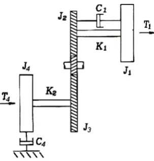
$x.

and

<f>2-

For

example.

[K]_+[M]_

E

(2.28)

where

_ =

and

=

-T

T

(2.30)

The

stiffness

matrix

is

and

the

mass matrix

is

[K}

M

An

A12

Kn

A22

Mi

l-h-2

M12

A/22

(2.31)

(2.32)

The

elements

of

the

stiffness

and mass matrices are

listed below.

An

/

%\GJ\i\dx

Jo

K12

A'22

ijj-.GJ'i-o

dx

/

VoGJv'-i

Jo

dx

where

Mi

/

4>ipJi>i

dx

Jo

M2

/

i'\pJv->dx

Jo

M22

/

fopJfo

dx

Jo

J

U^-y)

and

r0

and

r,

are

functions

of

x, the

distance along

the

length

of

the

shaft.

2.2.4

Formulation

of

System

Equation

of

Motion

2.2.4.1

Free

Vibration

Solution

To find

the

system's

free

undamped

vibration, the

following

differential

equation

of motion must

be

solved,

[M]s

0

+

8

₀

(2.34)

where

and

are

the

mass

and

stiffness matrices of

the system,

respectively.

For

a

linear

system,

0

(2.35)

where

0q

is

the

amplitude of

the

response.

Differentiating

Equation 2.35

twice

with

respect

to time

and

substituting into Equation 2.34

yields

(-u;2

+

[A]s)

0o

₀

(2.36)

The

natural

frequencies

of

the system, u>i,

can

be

expressed

by

solving

the

following

equation

for

det

(-a;,2

+

[A]s)

0

(2.37)

The

eigenvalues,

A,,

are

the

roots of

the system,

given

by

^

a;2

(2.38)

and

the eigenvectors,

fa,

are

the

displacement

vectors,

or

mode

shapes,

resulting

from

the

back

substitution

of

eigenvalues,

Aj.

2.2.4.2

Forced Vibration

Solution

can

be

represented

by

a vector.

m

[{fa},{fa},...,Un}\

(2.39)

The

orthonormal

modes,

or

the

weighted

normal

modes,

can

be determined

by dividing

the

normal

modes

by

the

square root

of

the

generalized

mass, Mu. The

generalized masses are

the

coefficients

of

the

identity

matrix,

so

that

mT[M}[}

[Mu}[I]

(2.40)

Therefore,

the

orthonormal

modal matrix elements

can

be

written

as

The orthogonality

relationships

are

[20]

:

and

where

[A]

Yi

sJ[Mu

[*r

[Af]

[*]

[I]

wr

[A]

[*]

[A]

Ai

0

0

0

0

A2

0

0

0

0

A3

0

0

0

0

Ar

(2.41)

(2.42)

(2.43)

(2.44)

In

matrix

form,

the

system equation of motion

for

the

continuous system

is

[Af]

{<?}

+

[C]

{0}

+

[A] {0}

{T}

(2.45)

where

the

[M], [C],

and

[A]

are

the mass,

damping,

and stiffness

matrices, respectively,

and

{T}

is

the

complex

torsional

forcing

vector.

The

system

damping

matrix,

[C],

from Equation

2.45,

can

be determined

by

decomposing

it

into

a

linear

combination

of

the

mass and stiffness

matrices

[18]:

[C]

a[M}+/3

[A]

where a and

j3

are coefficients

for frictional

damping

and structural

damping,

This

is

known

as

proportional

damping.

The

physical

coordinate,

0,

can

be

transformed

to

coordinate, q,

using

the

following

equation

[8]

{0}

[*]

{q}

(2.47)

Substituting

Equation

2.47 into 2.45

yields

[Af]

[*]

{q}

+

[C]

[$]

{q}

+

[A]

[*]

{q}

{T}

(2.48)

To

use

the

orthogonality

relationships,

Equations

2.42

and

2.43,

Equation 2.48 is

pre-multiplied

by

~-\T

-~iT

$

to

give

[*]

[M]

[$]

{q}

+

[C]

[*]

{q}

+

[A]

[$]

{9}

[$]'J'{T}

The

employment

of

equations

2.42,

2.43,

and

2.46 in 2.49

yields

[f] {?}

+

[a

[f]

+ /?

[A]] {q}

+

[A] {9}

[*]'

{T}

~lT

(2.49)

(2.50)

The

above

equation resembles

the

differential

equation of motion

for

forced

damped

vibration

in

terms

of

C,

the

damping

ratio,

and

ujn, the

natural

frequency

[20]

x

+ 2C^'x

+

F(t)

m

(2.51)

Therefore,

by

forcing

Equation 2.50

to

fit 2.51,

the

damping

coefficient

can

be

simplified

to

(a+^n;23)=2^m

(2.52)

The

system

damping

matrix

can

then

be

written with

the

diagonal

elements

being 2Qu)ni

[8]

[C]

0

0

0

2(>2

0

0

0

(2.53)

where

Ci

is

the

modal

damping

ratio

for

the

ith

normal mode.

where

c

is the

damping

constant,

and

cc

is

critical

damping

[18]

cc

2rrtaJni

(2.55)

If

lQ}

mT{T}

(2.56)

then

Equation 2.50 becomes

q,(t)

+

2c,-,--;ni.fc(*)

+

WnMt)

Qi(t)

(2.57)

after

substituting

Equations

2.52

and

2.56. When

the

modal

damping

ratio

is

less

than

1,

according

to

Rao

[18],

the

solution

to the

above

equation can

be

expressed as

qx

(t)

A

+

B +

C

(2.58)

where

A

e'^"'*

l

cosu;,7,-f

cosydlt

+

sin^f

>

qt

(0)

(2.59)

i-C

B

\

smudit

}

qx

(0)

(2.60)

C

/

Ql(T)e-Q-,"At-T)

sinu:di

(t

-t) dr

(2.61)

\jJdi

Jo

and

"'d,

=u.'ni-v/l-Ci

(2.62)

This

solution must

be

transformed

back

to

physical

coordinates

using

Equation

2.47.

2.3

Computer

Incorporation

and

Numerical Examples

Section 2.2

was

coded

into

a

FORTRAN

computer

program

called

FETORS.

Gauss-Legendre

Algorithm

was used

to

evaluate

the

eigenvalue solution.

FETORS

requires an

input

file

that

con

tains

the

torsional

system's

geometry,

as

well

as

any

other

necessary information

such

as

damping,

couplings,

external

torques,

and

lumped

external

inertias.

FETORS

is

capable of

evaluating

mul

tiple

rotor systems connected

by

couplings,

geared

rotor

systems

with

different

speeds,

and rotor

systems

with

different

material properties.

A

listing

of

the

FETORS

computer program

is

provided

in

Appendix C.l.

The

of

the

finite

element

torsional

formulation

embedded

in

FETORS

is demon

strated

by

using

the

program

to

determine

the torsional

natural

frequencies

and

mode shapes of

a

uniform

cylindrical shaft

and

a

tapered

shaft.

In

the

case

of

the

uniform

cylinder,

the

results

given

by

FETORS

are

compared

to

a

known

exact solution.

For

the tapered shaft, the

results

are

compared

with other

methods,

such as a stepped-cylinder model and

TAP.

Convergence

curves

for

the

first

two modes,

which

show

how many

elements

are

required

for

the

new

model

to

produce

accurate

results,

are

given

for

each

example

case.

Also,

two

additional

examples

are

presented

illustrating

the

forced

response analysis capabilities

of

the

computer program.

2.3.1

Uniform Free-Free

Shaft

A

uniform

(cylindrical)

free-

free

shaft was modelled

using

the

finite

element

formulation,

as a

series

of

"tapered

having

equal

left

and right end outer

diameters.

The

uniform

shaft

geometry is

as

follows:

L=

100 in.

D

10 in.

The

calculated natural

frequencies

and

mode

shapes of

the

uniform

free-free

shaft

determined

The

exact natural

frequency

of

a

uniform

free-free

shaft

in hertz

(Hz)

is

given

by

1

fi

(cGy

(263)

2irl

\

plp

J

where

A,

is the transcendental equation,

I

is

the

element

length,

C

is

the torsional

constant of

the

cross

section,

G

is

the

shear

modulus, p is

the

mass

density

of

the element,

and

Ip

is

the

polar

second

area moment of

area about

the

axis of

torsion,

as

given

below.

/

1,2,3...

A,

in

tvR4

C

G

h

2

E

2(1

+

!/)

vrA4

where

R

is

the

radius of

the

shaft.

The

exact mode

shape

is

given

by

the

expression

x\

fnrx\

l)

=

cos

vt)

{2M)

where

i

1, 2,

3

.,

x

is

the

axial position

along

the element,

and

I

is

the

element

length.

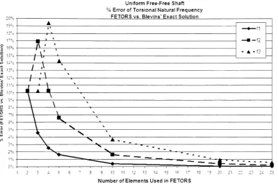
Figure 2.3

compares

the

first

three torsional

natural

frequencies,

as a

function

of

the

number

of

elements,

from FETORS

with

Blevins'

[6]

exact

solution.

FETORS

was run seven

times,

each

with

a

different

number of elements

representing the

100 inch

long

shaft.

The

results show

that

approximately ten

elements

are needed

to

predict

the

first

natural

frequency

within

1%

of

the

exact

20%

1?%

13%

17%

16%

11%

10%

3%

3%

Uniform Free-Free Shaft

% Error

Torsional Natural

Frequency

FETORS

Exact

Solution

?

J

-

A

-f3

,v

1

\'

1

*

/

A

\

/

'\

4

\

\

\

\

\

v_

\

<

\

s.

\

s.

\

x

A

-V.

-.

>

_

*- " "

-_

1 1 1 1 1 1 1 ,--4'f

v

v

0

1

2

9

10

13

15

18

Number

Elements Used in FETORS

19

20

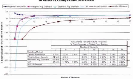
2.3.2

Tapered

Shaft

A

tapered

fixed-free

shaft

was

modelled

using

six

different

methods,

three

of which

were

in FE

TORS. The

three

different

modelling

methods

used

in FETORS

were

the

presented

finite

element

formulation,

and

two

stepped-cylinder models

based

on

different diameters

to

represent

a

tapered

element as

an equivalent uniform straight element.

The

other

modelling

methods were

TAP

[15]

and

ANSYS [1]. All

methods

were

compared

against

the

closed

form

solution

for

a

tapered

fixed-free

shaft,

or

truncated cone,

derived

by

H.D.

Conway

[11].

The

solid

metallic

tapered

shaft

had

the

following

material properties and

geometry,

which

equated

to

a

taper

angle of

11.31.

The

larger

diameter

end was

fixed,

while

the

other

end was

free.

E

29.5 Mpsi

u=

0.32

p

0.283

L

20 in.

DL

4 in.

DR

12 in.

2.3.2.1

FETORS

Three different

modelling

approaches

were

used

in

the

FORTRAN

program,

FETORS:

the ta

pered

finite

element

formulation,

and

two

stepped

cylinder

models

each with

a

different

method

of

determining

the

uniform

diameter

to

represent

the

tapered

element.

The

tapered geometry

was modelled

directly

using

the

new

finite

element

formulation,

with

increasing

number

of elements.

Stepped-Cylinder Model

Geometric Average

Diameter:

This

approach models

a

tapered

shaft

using

multiple numbers of uniform

cylindrical

beam

elements

in

series,

otherwise

known

as stepped-cylinder or stepped-shaft modelling.

The

geometric

average

of

the

elemental

left

and

right

end

diameters

was

taken to

be

the

equivalent

diameter

of

the

uniform section

representing

the tapered

element:

DL

+

Dr

Dequiv

5

(2-65)

Although

simple, this

approximation approach will yield error

in

the

mass

inertia

and stiffness of

the

stepped-cylinder

representation.

This

error

clearly

reduces with

increased

number of

elements

used

to

model

the tapered

shaft.

Stepped-Cylinder

Model

Weighted

Average

Diameter:

As

opposed

to the

geometric

average

diameter

model

described

above, this

approach

uses a

weighted average

diameter

to

represent

the

tapered

element

as a uniform

cylindrical,

or

straight,

element.

This

was achieved

by

forcing

the

uniform element

used

to

represent

the tapered

geometry

to

have

the

same mass

inertia

as

the tapered

element.

The

mass

inertia

of

a

tapered truncated cone,

or

frustum,

can

be

expressed as

'

m.D

I

where

f-

mV{x

,

L

(Z66>

m

pV

(2.61

7T

V

J

(2.68)

and

n(r\

Dr

r>r)

D(x)

DL

+

{DR

By

substituting Equation 2.68

into

2.66,

the

mass

inertia

of

the tapered

element

can

be

expressed

as

g/>M

(2.70)

The

mass

inertia

of

equivalent

uniform cylinder

is

t _

Pn \X>equiv)

>

t.-y

32

By

equating

the

mass

inertias

for

the

tapered

and

uniform

elements,

Equations 2.70

and

2.71,

the

diameter

of

the

equivalent uniform cylinder

is

V'equiv

fV

+

dl3dr

+

+

+

fV)

(2.72)

Although

this

approach

yields

an

equivalent

mass

inertia,

the

elemental

stiffness

is

only

approximated.

2.3.2.2

Torsional

Analysis Program-Holzer's Method

The

same

tapered

free-free

shaft

was

modelled

in

TAP,

Torsional

Analysis Program

[15].

This

method

is based

on a

distributed

point mass representation of

the

rotor's

inertial

con

nected

together

by

mass-less

elastic shaft

elements

that

behave

as

torsional

springs.

This

program

calculates

the torsional

natural

frequencies

and

modes

shapes

from

user-supplied mass

inertias

and

torsional

stiffnesses used

to

represent

the

rotor system.

In

this method,

the

mass

inertia

of

one

element

is

split

so

that

one

half

of

it is

distributed

on

the

left

end of

the torsional

spring

and one

half

is

on

the

right end.

Since

the

shaft

is

tapered,

the

mass

inertia

is

not constant

for

all elements.

The

mass

inertia

for

a

tapered

element

is

f'

mD

-f

Jo

dx

where

m

pV

(2.74)

and

V

(x)

and

D

(x)

are given

by

Equations

2.68

and

2.69.

Identical

to

the

weighted

average

diameter

case of

the

stepped-cylinder

model, the

equivalent

diameter

used

to

represent

the

tapered

element

as a uniform straight element

is

^equiv

fV

+

DL3DR

+

+

+

fV'

(2.75)

which

is

also

Equation

2.72.

Blevins

[6]

states

that the torsional

stiffness of

a

tapered

beam

can

be

calculated

by

K

^L

r^g

32

l

[Dr/Dl

+

+

(DR/DLf

2.3.2.3

ANSYS

The

tapered

shaft was modelled

twice

in

ANSYS

8.1

[1].

First,

three-dimensional tapered

elements

(Beam44)

were

used

to

model

the

fixed-free

shaft

using different

mesh

densities:

5, 10, 20, 25,

and

50

elements.

The

second

model

consisted

of

9720 20-noded

solid

brick

elements

(Solid95),

which

contained over

40,000

nodes.

It

must

be

noted

that

a

sensitivity study

was

conducted

on

the

density

of

the

mesh within

the

ANSYS-Solid95

model,

and

it

was

illustrated

that the

fundamental

and second

torsional

natural

frequencies

were

not affected when

the

number of

elements

used

in

the

model

were

increased.

This demonstrates

the

preciseness

of

this

model.

2.3.2.4

Results

and

Discussion

The first

and second

torsional

natural

frequencies

were

determined

using

each of

the

six

methods

solution

yields

a

fundamental

torsional

natural

frequency

of

2944.97

Hz,

and

a second

torsional

natural

frequency

of

5052.77 Hz.

The

ANSYS-Solid95

model

produced

corresponding

results

of

2978.2

and

5473.1

Hz.

Table

2.1:

Tapered

Fixed-

Free

Shaft: Fundamental Torsional

Natural

Frequency

NumberofElements

Modelling

Tapered Formulation 3.062.67 3,039.50 3.031.50 3.021.,00 3.017.83 3.01550 3.015.33 3.015.00 WeightedAvg. Diameter 2.513.83 2.778.17 - 2.927.83 2.993.83 3.010.50 3.012.17 3.014.17 Geometric Avg. Diameter 2.560.33 2.813.83 - 2.944.50 2.997.67 3.010.50 3.012.17 3.014.17 TAP 1.839.75 2,423.79 2.665.98 2.786.44 2.957.32 3.002.23 3.007.71 3.019.62

ANSYS-Solid95 2.978.2

ANSYS-Beam44

|

]

|

|

|

|

|

Table

2.2:

Tapered Fixed-Free Shaft:

Second

Torsional Natural

Frequency

NumberofElements

Modelling

Tapered Formulation 6.248.17 6.006 17 5.833.00 5.735.33 5.591.00 5.552.67 5.548.00 5.541.83 WeightedAvg. Diameter 4,377.17 5.104.50 - _5.443.17

5.521.83 5.537.83 5.538.50 5.539.50

Geometric Avg. Diameter 4,322.50 5,104.50

-5.458.50 5.529.33 5.537.83 5,538.50 5.539.50 TAP 2.626.75 3,707.61 4.415.41 4.794.31 5.345.97 5,494.29 5,512.25 5.539.82

ANSYS-Solid95 5.473.1

ANSYS-Beam44

|

|

|

|

|

|

The

natural

frequencies

were compared

to

Conway's

closed

form

solution,

and

the

correspond

ing

errors are presented

in

Figures

2.4

and

2.5.

Note

that the

results

from

the

ANSYS-Solid95

model

are plotted

as

a single

line for

reference.

It

was

found

that the two

stepped-cylinder

models,

Weighted Average Diameter

and

Geo

metric

Average

Diameter,

yield

remarkably

similar results.

Nevertheless,

these

results

demonstrate

the

level

of

inaccuracy

introduced

with

a

stepped-cylinder

approximation

to modelling

a

tapered

shaft.

Moreover,

the

FETORS

tapered

element model

monotonically

converges

to the

closed

form

solution

from

above, consistently overestimating the

solution.

This

is

a

desirable

characteristic

since