Goodness-of-fit test in parametric mixed effects models based on estimation of the error distribution

(1)

City, University of London Institutional Repository

Citation: González-Manteiga, W., Martinez-Miranda, M. D. & Van Keilegom, I. (2016).

Goodness-of-fit test in parametric mixed effects models based on estimation of the error distribution. Biometrika, 103(1), pp. 133-146. doi: 10.1093/biomet/asv061

This is the accepted version of the paper.

This version of the publication may differ from the final published

version.

Permanent repository link: http://openaccess.city.ac.uk/17075/

Link to published version: http://dx.doi.org/10.1093/biomet/asv061

Copyright and reuse: City Research Online aims to make research

outputs of City, University of London available to a wider audience.

Copyright and Moral Rights remain with the author(s) and/or copyright

holders. URLs from City Research Online may be freely distributed and

linked to.

(2)

Goodness-of-fit Test in Parametric Mixed Effects Models

based on Estimation of the Error Distribution

BY WENCESLAO GONZ ´ALEZ-MANTEIGA

Department of Statistics and Operations Research, University of Santiago de Compostela, Faculty of Mathematics, 15782 Santiago de Compostela (Spain) 5

[email protected]

MAR´IA DOLORES MART´INEZ-MIRANDA

Department of Statistics and Operations Research, University of Granada Campus Fuentenueva s/n, 18071 Granada (Spain)

[email protected] 10

ANDINGRID VAN KEILEGOM

Universit´e catholique de Louvain

Voie du Roman Pays, 20, B-1348 Louvain-la-Neuve (Belgium)

[email protected]

SUMMARY 15

We address the problem of testing for a parametric function of fixed effects in mixed mod-els. We propose a test based on the distance between two empirical error distribution functions, which are constructed from residuals calculated under the opposing hypotheses. The proposed test statistic has power against all alternatives, and its asymptotic distribution is derived. A

sim-ulation study shows that the test outperforms others in the literature. The test is applied to longi- 20

tudinal data from an AIDS clinical trial and a growth study.

Some key words: Bootstrap; Empirical distribution; Residual; Local polynomial estimation; Mixed model.

1. INTRODUCTION

Mixed effects models assume a flexible covariance structure which allows for non-constant

correlation among the observations, and have become very popular for many practical situations. 25

A mixed effects model, or simply mixed model, contains both fixed and random effects. While the former describe the relationship between the covariates and the response for all the obser-vations, the latter are specific to clusters or subjects within a population. This kind of model is suitable for problems related to, e.g., longitudinal data, repeated measurements, clustered data

and small area estimation. 30

The most popular parametric mixed effects models are linear mixed models or generalized linear mixed models, which can be described as

g{E(Yij |Xij, bi)}=m(Xij) +bTiZij, (1)

where, g is a known link function, Yij is the response variable, Xij is a covariate vector of

(3)

2 W. GONZALEZ-MANTEIGA, M.D. MARTINEZ-MIRANDA ANDI. VANKEILEGOM

bi is a d′-dimensional vector of mean zero corresponding to the random effects. Whengis the

35

identity function and mis linear we have the linear mixed model. The nonlinear mixed model

arises when the right-hand side in equation (1) is a nonlinear function of the fixed and random effects; see Pinheiro & Bates (2000).

The parametric assumption simplifies both theoretical and computational aspects, but it also provides valuable interpretations in real data applications. Therefore, it is of interest to test the

40

adequacy of simple parametric mixed models. There are different approaches to test parametric

assumptions for the function of the fixed effects, given by the functionmin model (1), or for the

distribution of the random effects, typically considered to be normally distributed.

Specification tests for the function m in model (1) are well-established in the literature in

the absence of random effects. Different methods developed in the last twenty years

(Gonz´alez-45

Manteiga & Crujeiras, 2013) can be classified into three groups: tests based on the comparison between nonparametric and parametric estimates; generalized likelihood ratio tests; and tests based on the empirical distribution of the residuals. Contributions for the case with random ef-fects are more recent and scarce. Zhang & Lin (2003) consider a test for a semiparametric

addi-tive mixed model, wheremis an additive function. In particular, when one additive component

50

is linear and the other is nonparametric, they designed a goodness-of-fit test for polynomial re-gression in the nonparametric component. The authors assume clustered normal and non-normal data and base the test on nonparametric estimation by smoothing splines. Lombard´ıa & Sperlich (2008) propose a test based on kernel smoothing to check a linear function for the nonparamet-ric component of a generalized semiparametnonparamet-ric additive model. See also Sperlich & Lombard´ıa

55

(2010), which is motivated by the small area estimation problem, and Henderson et al. (2008). In the context of linear mixed models, or generalized linear mixed models, recent papers ex-ploit the link between random effects and penalized regression, developing restricted likelihood ratio testing for zero variance components in linear mixed models. These methods, which are

extensions of theF-test, have been applied to test whether the fixed effects are linear, quadratic,

60

cubic, etc., in the presence of random effects, see Greven et al. (2008) and Wood (2013a,b). Huet

& Kuhn (2015) suggest an omnibus test that exploits the ideas of theF-test but using a

Bonfer-roni adjustment. Lin et al. (2002), Pan & Lin (2005) and S´anchez et al. (2009) provide omnibus tests for linear mixed models and generalized linear mixed models, based on cumulative sums of the residuals with respect to the covariates or the predicted values.

65

On the other hand, inference about the assumptions made for the random effects in model (1),

for example the normal distribution of thebi’s, has been considered recently in many papers. See

Claeskens & Hart (2009) for an extensive review, or Meintanis & Portnoy (2011).

In this paper we propose a test based on the empirical distribution of the residuals. It extends the test of Van Keilegom et al. (2008), who consider a model without random effects representing

70

cross-sectional independent data. This kind of method is very powerful, since it can detect alter-natives at the parametric raten−1/2_{. To calibrate the distribution of the test statistics we suggest}

a bootstrap method suitable for the assumed mixed effects model.

2. MODEL AND ESTIMATION

In this paper we consider the semiparametric one-way model

75

Yij =m(Xij) +bTi Zij +ǫij (j= 1, . . . , ni; i= 1, . . . , q), (2)

where q is the number of levels in the model and n=Pq_i₌₁ni is the total number of

ob-servations. The covariate Xij is a d-dimensional random vector, and Zij is a sub-vector of

(1, XT

(4)

FX and density fX, and X1, . . . , Xq are mutually independent, with Xi = (Xi1, . . . , Xini)

T_.

We assume that the errorsǫ11, . . . , ǫqnq are independent and identically distributed normal ran- 80

dom variables with mean zero and varianceσ2_{, and that}_E₍_ǫ

ij |Xij) = 0. The random effects

b1, . . . , bq are independent and identically distributedd′-dimensional normal random variables

with mean zero and covariance matrix Vb, which quantifies the within-subject variation.

Fur-ther, assume that bi andXi′ are independent for i, i′= 1, . . . , q, so b_i is independent of X_i. Moreover, cov(bi, ǫi′_j |X_i, X_i′) = 0 for alli, i′ = 1, . . . , qandj= 1, . . . , n_i′. The normal as- 85

sumption made for the random effects and the errors could be relaxed (Severini & Staniswalis, 1994; Lin & Carroll, 2000). Here we make this assumption to develop simpler likelihood-based inferences for the functionm, as well as for the estimation of the variancesVbandσ2.

Since the observations are only dependent if they come from the same individual, we can

write (2) using matrix notation. Thus we first stack the observations at the individual level, i.e., 90

Yi =m(Xi) +Zibi+ǫi(i= 1, . . . , q), whereZiis theni×d′matrix with rowsZiT1, . . . , ZinTi,

Yi = (Yi1, . . . , Yini)

T_{, and}_ǫ

i = (ǫi1, . . . , ǫini)

T _{has diagonal covariance matrix}_σ2_I

ni. Also, the

variance ofYiconditionally onXiis

Vi =ZiVbZiT +σ2Ini. (3)

The model can be compactly written for the whole set ofnobservations asY =m(X) +Zb+ǫ,

whereY = (YT

1 , . . . , YqT)T,Xis then×dmatrix with rowsXiT, andZ is then×qd′ matrix 95

with diagonal blocks Zi. Here, the variance of Y conditionally on X is V =ZBZT +σ2In,

whereBis the matrix with diagonal blocksVb.

Under a parametric mixed effects model the function of the fixed effects m is commonly

estimated by the global likelihood method. Under the above conditions the density of Yi,

conditionally onXi, is normal with mean m(Xi) ={m(Xi1), . . . , m(Xini)}

T _{and covariance}

100

matrixVi. Then the log-likelihood ofY conditional onXis

ℓ(m, Vb, σ2) =− 1 2

q

X

i=1

h

{Yi−m(Xi)}T V_i−1{Yi−m(Xi)}+ log|Vi|+ 2nilog(2π)

i

. (4)

Here we are interested in estimating m(x), for any fixed x inRd, by a local polynomial

ap-proach. We consider an extension of the common local polynomial estimator for independent and

identically distributed data, derived using local likelihood. For a givenxand supposing thatXij 105

is close toxand thatmis continuous atx, we have thatm(Xij)≈m(x) =βx0(j= 1, . . . , ni).

Model (2) can then be locally approximated by the mixed modelYi =Pi(βx, x, p) +Zibi+ǫi,

wherePi(βx, x, p)is ani-dimensional vector of polynomials of orderpcontaining all products

of factors of the formXij,ℓ−xℓ(ℓ= 1, . . . , d;j= 1, . . . , ni). The vectorβxconsists of all

co-efficients of these polynomials, and its first component isβx0 =m(x). The local log-likelihood 110

can be defined from the global log-likelihood (4), by introducing local weights for each observation. However, in the presence of within-subject correlation in the model, this should

be done using blocks, i.e., considering each of the q independent components of the global

log-likelihood. As Lin & Carroll (2000) pointed out, the way to introduce the kernel weights

into the individual components is problem-specific, and different ways provide estimators with 115

(5)

ℓloc(βx, Vb, σ2) =− 1 2

q

X

i=1

{Yi−Pi(βx, x, p)}TW_ih,x1/2Vi−1W

1/2

ih,x{Yi−Pi(βx, x, p)}

+ log|Vi|+ 2nilog(2π), (5)

where the matrixWih,xis diagonal with elementsKh(Xij−x)for each independent block (i=

120

1, . . . , q). Here, for u= (u1, . . . , ud)∈ Rd, K(u) =Qd_j₌₁k(uj) is a d-dimensional product

kernel, k is a univariate kernel function,h≡hn is a bandwidth sequence converging to zero

whenntends to infinity, andKh(u) =Qdj=1{k(uj/h)/h}. The estimatormb(x)is then defined

as the first component of the vector that maximisesℓloc(βx, Vb, σ2)overβx.

For the special case of local linear smoothing, i.e., when p= 1, the

estima-125

tor m_b(x) can be explicitly written as the first component of the 2×1 vector

Pq

i=1XiTW

1/2

ih,xV

−1

i W

1/2

ih,xXi

−1Pq

i=1XiTW

1/2

ih,xV

−1

i W

1/2

ih,x Yi, withXi being theni×2

ma-trix with rows (1, Xij −x)T (j = 1, . . . , ni; i= 1, . . . , q). The local constant case, p= 0, is

analogous but replacing the matrixXiby theni-dimensional vector of ones,1ni. If there is no

within-subject correlation, or it is ignored, the derived estimator for m(x) is the local linear

130

estimator for independent data whenp= 1, and the Nadaraya–Watson estimator whenp= 0.

Since the estimator ofm(x)depends onVbandσ2, which are unknown in general, the

corre-sponding feasible or empirical estimator at eachxcan be derived using a three-step procedure.

The procedure accomplishes the estimation ofβ and the variancesVbandσ2, using

simultane-ously the local and global log-likelihoods (5) and (4), and is formulated as follows:

135

Step 1. For arbitrary values of σ2 and Vb define the estimator of m(x) for any x by

b

mσ,Vb(x) =βbσ,Vb, which is the first component of the maximizer ofℓloc(βx, Vb, σ

2₎_.

Cal-culatem_bσ,Vb(Xij)for all observedXij’s.

Step 2. Compute the estimator of(Vb, σ2)as the maximizer(Vbb,σb2) ofℓ(mbσ,Vb, Vb, σ

2₎_{, from}

the global log-likelihoodℓ(m, Vb, σ2)given in (4).

140

Step 3. Finally, computem_b(x) =βb_b

σ2

,Vbb.

From m_b(Xi) ={mb(X1), . . . ,mb(Xq)}T, the random effectsbi can be predicted using

stan-dard methods for linear mixed models bybbi =VbbZiTVb

−1

i {Yi−mb(Xi)}(i= 1, . . . , q).

The above three-step procedure is suitable for model (2), where σ2 and Vb are global

pa-rameters, and β is the only local parameter, but it can be easily adapted depending on which

145

parameters in the model are global and which ones are local. For example, if the model is het-eroscedastic, i.e., var(ǫij |Xij) =σ2(Xij), then we could estimateσ2(·)in the first step of the

above procedure. Then we would maximize the local log-likelihood at each point x, with

re-spect to βx, σ2(x) and Vbb(x). We could also consider that m belongs to a parametric class

M={mθ :θ∈Θ}, in which case the estimation ofm would move to the second step of the

150

procedure. Then, we would maximize the global log-likelihood with respect toθ,σ2andVb.

Fi-nally, note that our three-step procedure can be applied with any local log-likelihood and hence

to any local estimator ofmproposed in the literature. If the error is not supposed to be normal,

steps 1 and 2 could be based on a quasi-likelihood approach and on general estimating equations, see, e.g., Liang & Zeger (1986) and Lin & Carroll (2000).

(6)

3. GOODNESS-OF-FIT TESTING

In this section we propose a test for the parametric null hypothesis about the function of the

fixed effectsm, formulated as follows:

H0 :m∈ M={mθ : θ∈Θ}, H1 :m /∈ M, (6)

whereΘis a compact subset ofRs_{. Let}_θ

0be the true value ofθunderH0, which is supposed to

belong to the interior ofΘ. UnderH1, let us defineθ¯as the minimizer ofE[{m(X)−mθ(X)}2] 160

inΘ. Note thatθ¯=θ0underH0. The proposed test extends that of Van Keilegom et al. (2008)

for cross-sectional independent data. The first step in defining it is to characterize the null hy-pothesis; see Theorem 2.1 in Van Keilegom et al. (2008). This result is based on the comparison between the error distributions under the null and the alternative hypotheses. When the regression

model involves random effects, we can consider two approaches depending on how we define the 165

errors: either the marginal errors,Uij =Yij−m(Xij), arising from the marginal distribution of

the responseYij, or the conditional errors,ǫij =Yij −m(Xij)−bT_i Zij, arising from the whole

regression structure, i.e., the distribution conditional on the random effectsbiand the covariates.

Inference from conditional errors requires the estimation of both the random and the fixed

ef-fects, but the results of the tests can be affected by misspecification of the random component 170

(Pan & Lin, 2005). The whole regression model is the target for testing procedures based on conditional residuals. However, our goal is to test the function of the fixed effects, so we suggest a test based on the marginal errors.

Consider the marginal errorsUij =Yij−m(Xij). Such errors are not independent and

iden-tically distributed, so the assumptions in Van Keilegom et al. (2008) do not apply. In or- 175

der to remove the within-subject correlation, such errors have to be standardized. We

con-sider the block transformationV−1/2_U_{, based on the whole vector}_U _{= (}_UT

1 , . . . , UqT)T, with

U_iT = (Ui1, . . . , Uini). The elements ofV

−1/2_U _{are then independent and identically distributed}

variables, so we can follow arguments like those in Van Keilegom et al. (2008) to formulate

the test statistics. Let us denote the elements of the transformed vector of errors by U′

ij, and 180

note that they all have the same distribution as a generic variableU′

. Analogously, consider the transformed errors based on the parametric regression function under the null hypothesis, i.e.,

V−1/2_{_Y ₋_m ¯

θ(X)}, with elements denoted byUij,′ 0, which are also independent and

identi-cally distributed variables with the same distribution as U′

0, under H0. From these definitions

the characterization of the null hypothesis in problem (6) follows by using arguments from Van 185

Keilegom et al. (2008). This is formulated in the next proposition, whose proof is given in the Supplementary Material.

PROPOSITION1. Letmbe a continuous function. The null hypothesisH0:m∈ Min (6) is

valid if and only if the standardized marginal errorsU′ andU′

0have the same distribution.

The next step is to estimate the distribution of the random variables U′ _and_U′

0, which we 190

denote byFU′ andF_U′

0; we assume that their corresponding densities exist and denote them by

fU′andf_U′

0 respectively. We consider the estimators ofmand the varianceV resulting from the

three-step estimation method presented in Section 2. Denote these estimators bym_b andVb, where

b

V is the block diagonal matrix with blocksVbi =ZiVbbZiT +σb2Ini. Then we can estimate the

dis-tribution ofU′ _{by the empirical distribution of the standardized nonparametric marginal}

resid-195

uals, FbU′(t) =n−1P_iq₌₁Pn_j₌₁i I Ub_ij′ ≤t

.Here, the Ub′

ij’s denote the elements of the vector

b

V−1/2_{_Y ₋_m_b₍_X₎_}_{, and}_I _{is the indicator function. In the case of independent and identically}

(7)

Keilegom (2001) for the special case whered= 1andp= 0, and by Neumeyer & Van Keilegom

(2010) for the general case. Also, the distribution ofU′

0is estimated by the empirical distribution 200

of the parametric marginal residuals Ub′

ij,0, i.e., FbU′

0(t) =n

−1Pq

i=1

Pni

j=1I Ub

′

ij,0 ≤t

,where

theUb′

ij,0’s are defined as the elements of the vector Vb

−1/2_{_Y ₋_m_b

0(X)}. The estimatormb0 is

defined analogously to m_b, but replacing the observed responsesYij by the parametric

estima-tor m_b_θ(Xij) of the fixed effects. Here the estimatorθbcan, e.g., be defined by maximizing the

global likelihoodℓ(mθ, Vb, σ2)with respect toθ,Vbandσ2, but other estimators are possible if

205

assumptions (A7) and (A7⋆) below are satisfied.

Finally, we measure the distance between the empirical distributions FbU′ and Fb_U′

0, using Kolmogorov–Smirnov and Cram´er–von Mises type statistics,

Tn,KS=n1/2 sup

−∞<t<∞

bFU′(t)−Fb_U′

0(t)

, Tn,CM=n

Z n b

FU′(t)−Fb_U′

0(t)

o2

dFb_U′

0(t).

To study the local power of these statistics, we consider the local alternatives

210

H1n:m(·) =mθ0(·) +n

−1/2_r₍_·₎

for some bounded functionr. These alternatives only concern the regression function and not the

error distribution. The main asymptotic result of this paper provides the asymptotic distribution

of the two test statistics. The result, given in Theorem 1 below, is formulated underH1n, but it

also coversH0by taking the functionrequal to zero. We need the following assumptions:

215

(A1) the number of blocks,q, tends to infinity, andni≤C(i= 1, . . . , q), for someC <∞;

(A2)nh2p+2→0ifpis odd,nh2p+4 →0ifpis even, andnh3d+ν → ∞for some smallν >0;

(A3)kis a symmetric probability density function supported on[−1,1],kisd-times

continu-ously differentiable, andk(j)₍_±_{1) = 0}₍_j_{= 0}_{, . . . , d}₋₁_);

(A4) all partial derivatives ofFXup to order2d+ 1exist on the interior of the compact support

220

RX ofX, they are uniformly continuous, andinfx∈RXfX(x)>0;

(A5) all partial derivatives ofx→m(x)up to orderp+ 2exist on the interior ofRX, and they

are uniformly continuous;

(A6) all partial derivatives of (x, θ)→mθ(x) up to order2exist on the interior of RX ×Θ,

and they are continuous in(x, θ); and

225

(A7) the estimator θb can be written as θb−θ0 =n−1Pq_i₌₁P_jn₌₁i ξ(Xij, Yij)+n−1/2δ+

oP(n−1/2), where ξ satisfies E{ξ(Xij, Yij)|Xij}= 0 both under H0 and H1n.

More-over, the asymptotic distribution ofn−1/2Pq

i=1

Pni

j=1ξ(Xij, Yij) underH0 is the same

as under H1n, and the constantδ depends on the direction of the alternative hypothesis

determined by the functionr, and equals zero underH0.

230

Assumption (A1) is common in the context of mixed effects models. In the context of longitudi-nal data it states that the number of individuals increases but the number of observations for each individual is bounded. Assumptions (A2)–(A5) come from Neumeyer & Van Keilegom (2010) and are required to obtain the asymptotic distribution of the processn1/2_{_F_b

U′(·)−F_U′(·)}. As-sumption (A6) is necessary for applying the asymptotic results in Van Keilegom et al. (2008).

235

Finally, (A7) is needed to decompose the processn1/2{FbU′

0(·)−FU′(·)}into a sum of indepen-dent and iindepen-dentically distributed terms and negligible terms, from which the weak convergence of this process will follow. See also Pan & Lin (2005), formula (2), and Theorem 3.1.2 in the 1994 Wisconsin-Madison University PhD thesis by J. C. Pinheiro, for similar decompositions, and for precise conditions under which this assumption holds true.

(8)

We are now ready to state the main result describing the limiting distribution of the test

statis-ticsTn,KSandTn,CM. The proof forp= 0andp= 1is given in the Supplementary Material.

THEOREM1. Assume that conditions (A1)–(A7) are satisfied. Then, underH1n,

Tn,KS→ sup

−∞<t<∞

|fU′(t)| |W −a|, T_n,_CM → Z

f_U2′(t)dFU′(t) (W −a)2

in distribution, whereW is a zero-mean normal random variable with variance given in equation 245

(5) in the Supplementary Material, and where the constant adepends on the direction of the alternative, defined also in the Supplementary Material, equation (4). Note thata= 0underH0.

Since the above limiting distributions are rather complicated, we suggest using bootstrap meth-ods to approximate the critical values. More precisely, we define a bootstrap algorithm suitable

for the assumed mixed model: 250

1. Calculate the estimator m_b of the function of the fixed effects m, the estimators Vbb andσb2

of the variancesVb andσ2, and also the estimatorm_b_θ of the parametric regression function

underH0. These estimators are derived using the three-step method in Section 2.

2. Generate bootstrap conditional errorsǫ⋆_ij independently from a normal distribution with mean

zero and varianceσ_b2, and bootstrap random effectsb⋆_i from ad′

-dimensional normal distribu- 255

tion with mean zero and covariance matrixVbb.

3. Under the null hypothesis the bootstrap responses are constructed by Y_ij⋆ =m_b_θ(Xij) +

(b⋆_i)TZij +ǫ_ij⋆ (j= 1, . . . , ni; i= 1, . . . , q). Then, the bootstrap sample is given by

{(Xij, Zij, Yij⋆), j= 1, . . . , ni,i= 1, . . . , q}.

4. Calculate the bootstrapped test statisticsT_n,⋆_KS andT_n,⋆_CMfrom the bootstrap sample gener- 260

ated in the previous step.

Finally, the quantiles of the distribution ofT⋆

n,KSandTn,⋆CMcan be approximated by repeating

steps 2–4 in the bootstrap algorithmBtimes.

The resampling scheme could also be defined without using the normal assumption. In that

case both the conditional residuals and the random effects in the second step above could be 265

generated from the smoothed empirical distribution of the residuals (Van Keilegom et al., 2008). The consistency of this bootstrap procedure is shown in the next result and the proof is given in the Supplementary Material. For this, we need to introduce the bootstrap counterpart of (A7):

(A7⋆) underH0, the estimatorθb⋆ can be written asθb⋆−θb=n−1Pq_i₌₁Pn_j₌₁i ξ⋆(Xij, Yij⋆) +

oP⋆(n−1/2), in probability, whereξ⋆ satisfiesE{ξ⋆(X_ij, Y⋆

ij)|Xij}= 0and where

sup t

pr⋆nn−1/2

q

X

i=1

ni

X

j=1

ξ⋆(Xij, Yij⋆)≤t

o

−prnn−1/2

q

X

i=1

ni

X

j=1

ξ(Xij, Yij)≤to→0,

in probability.

THEOREM2. Assume that conditions (A1)–(A7) and (A7⋆) are satisfied. Then, underH0,

sup s

pr⋆(T_n,⋆_KS ≤s)−pr(Tn,KS≤s)

→0, sup

s

pr⋆(T_n,⋆_CM ≤s)−pr(Tn,CM≤s)

→0,

in probability, where the probability pr⋆is computed under the bootstrap distribution conditional 270

(9)

4. SIMULATION EXPERIMENTS

We simulate two different models: a simple model with just a random intercept,

Yij =m(Xij) +bi+ǫij, (7)

and a model with random effects consisting of a random intercept and a random slope, 275

Yij =m(Xij) +bi0+bi1Xij +ǫij. (8)

Both are particular cases of (2), withZij = 1for (7) andZij = (1, Xij)T for (8). In both cases

we considerXijto be scalar and generated from either a uniform distribution on[0,2]or a normal

distribution with mean zero and variance0.6. The random effects and the errorsǫij are generated

independently. The random effectsb1, . . . , bqin (7) are generated from a normal distribution with

280

mean zero and standard deviationσb0. We consider the valuesσb0 = 0.6, case 1, andσb0 = 1, case 2. The two-dimensional random vector(bi0, bi1)T (i= 1, . . . , q), in model (8), is bivariate

normal with covariance matrix Vb =diag(0.32,0.32). The errors are generated from a normal

distribution with mean zero and standard deviationσ= 0.3. We consider samples of sizesn=

150,300and600, where the number of observations per group is alwaysni = 3, and the number

285

of groups equalsq = 50,100and200. We test whether the function mis linear using the test

statisticsTn,KSandTn,CM.

The test involves a kernel estimator depending on three choices: the bandwidth parameter,h,

the degree of the polynomial,p, and the kernel function k. The asymptotic analysis shows that

the bandwidthhshould satisfy the conditions described in assumption (A2). We have considered

290

bandwidths of the type h=h0n−3/10, which satisfy this assumption, where h0 is a constant

value chosen around the range of the covariate X. This recommendation is similar to that of

Pardo-Fern´andez et al. (2007), who suggested the same kind of test in a different regression framework. In the Supplementary Material we analyse the sensitivity of the test to the bandwidth

choice using several values forh0 around the range of the simulated covariate values. The

con-295

clusion is that the test is quite robust to this choice so here we only report the caseh= 3n−3/10_.

Regarding the degree of the polynomial, it is known that the local linear estimator, p= 1, has

better properties than the local constant estimator,p= 0; see for example Wand & Jones (1995).

The effect of this choice is not major though; see the Supplementary Material. In this section, and in our other empirical analyses, we only consider the local linear case. Finally, it is

well-300

known that the choice of the kernel functionkdoes not have a major impact on the performance

of the kernel estimator (Wand & Jones, 1995), and therefore on our test. In our empirical studies

we consider the Epanechnikov kernel. We work with these choices ofh,pandkin the rest of

this section and derive the kernel estimator using the three-step estimation method presented in Section 2. We have approximated the critical values in the test using the bootstrap algorithm

305

described in Section 3 with B= 1000bootstrap samples. The bootstrapped test statistics have

been calculated using the choices ofh,pandkabove.

We consider two other tests that can deal with the formulated problem: the omnibus test of Pan & Lin (2005), which competes with our test if the aim is to test a linear mixed model, is based on the cumulative marginal residuals and has critical values obtained using an asymptotic

310

approximation valid for large values ofq; and the restricted likelihood ratio test of Greven et al.

(2008), which is not omnibus in the sense that a single test is performed to detect deviations from a null hypothesis. One can expect that the restricted likelihood ratio test, which is an extension

of the F-test, performs better than an omnibus test if the null hypothesis is linear. We have

calculated this test using the function exactRLRT in the R-package RLRsim (Scheipl et al., 2008).

315

(10)

bym(X) = 1 +X. Here, the considered nominal level isα= 0.05. The power was calculated by simulating also 1000 samples from two specific alternatives. The first consists of

contami-nating the null hypothesis with a sinusoidal function, by simulatingm1(X) = 1 + (1−a)X+

320

asin(πX), witha= 0.1and0.2. The second is harder to detect and allows us to check the power

against quadratic terms by simulatingm2(X) = 1 + (1−a)X+aX2 fora= 0.1and0.2. In

both cases, the valuea= 0corresponds to the null hypothesis of linearity.

Table 1 shows the results obtained from each test under this scenario and considering only

the normal design, which is also the most favourable design for the omnibus test of Pan & Lin 325

(2005). We considered a randomized rule (Pearson, 1950) to determine the rejection levels for

Tn,KS, which is discrete. This consists of deciding the rejection of the null hypothesis based

on a random experiment when the test statistic equals the approximated critical value. In our case we define the functionφα(s) ={αB−#(Tn,∗KS> s)}/#(Tn,∗KS=s), generate a uniform

numberu∈(0,1)and reject the null hypothesis ifu < φα(Tn,KS), or accept it otherwise. Here 330

the notation#(S)represents the cardinality of the setS. All the tests have similar empirical level for all sample sizes, and the average p-value of the test of Greven et al. (2008) is, in all cases, much higher than the expected value of 50%.

The power of the tests for the two alternatives are also shown in Table 1. Our test clearly

outperforms that of Pan & Lin (2005). The restricted likelihood ratio test has the highest power, 335

[image:10.595.143.467.453.686.2]

as expected since it incorporates model information. Taking this into account, we can conclude that our tests, in particular the Cram´er–von Mises test, have good power.

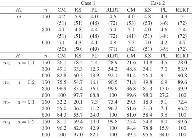
Table 1. Empirical size and power (%) of tests under two types of

alter-natives for model (7). Under the null hypothesis,m(X) = 1 +X, the av-erage p-value (%) is shown between brackets. The nominal level is 5%.

Case 1 Case 2

H0 n CM KS PL RLRT CM KS PL RLRT

m ₁₅₀ _4.2 _5.9 _4.0 _4.6 _4.0 _4.8 _4.3 ₅

(51) (51) (46) (72) (53) (53) (46) (72)

300 4.1 4.8 4.4 5.4 5.1 4.0 4.6 5.4

(51) (51) (48) (72) (41) (51) (48) (72)

600 5.1 4.3 4.1 4.8 5.2 5.0 4.2 4.7

(50) (50) (49) (71) (42) (51) (49) (72)

H1 n CM KS PL RLRT CM KS PL RLRT

m1 a= 0.1 150 26.1 18.5 5.4 28.9 21.6 14.8 4.5 28.0

300 49.1 33.3 12.3 54.2 48.8 34.1 7.0 53.9

600 82.8 60.3 18.9 92.1 81.4 56.4 9.1 90.8

m1 a= 0.2 150 75.5 54.7 16.1 90.5 71.8 49.8 6.9 89.6

300 96.9 85.4 36.1 99.9 96.8 81.3 15.0 99.9

600 100 97.7 68.8 100 99.6 98.0 27.2 100

m2 a= 0.1 150 32.2 20.1 7.3 73.4 29.5 18.9 5.1 72.4

300 55.0 36.5 11.2 96.2 51.6 31.3 7.4 96.2

600 84.3 55.7 24.0 100 81.0 58.4 9.6 100

m2 a= 0.2 150 81.1 59.4 19.0 99.8 75.4 54.8 8.0 99.6

300 96.2 82.9 42.9 100 94.4 78.8 15.9 100

600 100 97.0 82.1 100 99.5 95.6 34.0 100

(11)

[image:11.595.155.421.160.394.2]

Table 2. Empirical size and power (%) of tests under four

types of alternatives for model (8). Under the null hypothesis, m(X) = 1 +X, the average p-value (%) is shown between

brackets. The nominal level is5%.

Uniform Normal

H0 n CM KS RLRT CM KS RLRT

m ₁₅₀ _4.5 _4.2 _5.0 _4.8 _4.3 _6.5

(52) (51) (74) (51) (51) (71)

300 4.6 5.3 5.1 5.5 5.1 4.4

(48) (48) (73) (49) (50) (71)

600 5.7 5.4 5.0 3.9 3.8 5.2

(51) (51) (73) (49) (49) (73)

H1 n CM KS RLRT CM KS RLRT

m1 a= 0.2 150 17.9 14.3 35.9 24.8 21.4 58.2

300 33.9 24.8 70.0 53.5 47.4 91.6

600 49.9 43.3 95.4 81.9 73.2 99.6

m2 a= 0.2 150 9.5 11.8 23.6 31.2 33.2 66.7

300 16.8 19.1 47.8 65.0 66.7 93.1

600 27.0 29.5 77.7 90.5 91.0 99.6

m3 a= 0.2 150 24.1 17.5 38.2 74.2 60.3 90.5

300 34.9 27.2 66.7 93.6 85.5 99.6

600 49.6 42.2 93.7 99.7 98.8 100

m4 a= 0.2 150 9.3 11.3 20.9 27.0 22.0 39.0

300 12.1 13.3 42.2 43.7 37.6 68.4

600 18.9 20.4 72.8 64.0 58.6 94.2

CM, Cram´er–von Mises; KS, Kolmogorov–Smirnov; RLRT, Greven et al. (2008);m1(X), sinusoidal;m2(X), quadratic;m3(X), absolute value; m4(X), discontinuous.

To finish this section, we consider model (8). The power was calculated from four alternatives:

the samem1(X)andm2(X)considered above witha= 0.2, and non-smooth alternatives

de-fined by m3(X) = 1−a|0.5−X|andm4(X) = 1−aX I X≤0.5+a I X >0.5, also 340

witha= 0.2. Table 2 shows that for model (8) the size of our test is around the nominal level of

5% and the test provides reasonable power. We have not considered the test of Pan & Lin (2005) since it has been clearly beaten by our test in the simpler model (7). As expected, the test of Greven et al. (2008) exhibits the highest power but provides an average p-value, under the null hypothesis, much higher than 50%.

345

5. APPLICATION TOAIDSCLINICAL TRIAL

Our first application consists of CD4 counts data from an AIDS clinical trial to evaluate the efficacy of Zidovudine in treating patients with mild symptomatic HIV infection. These data have

also been analysed by Lin et al. (2002) and Pan & Lin (2005). A total of711patients enrolled

in the study, with 361 randomized to Zidovudine and 350 to placebo. Here we only consider the

350

(12)

0 10 20 30 40

0

200

400

600

800

1000

1200

1400

weeks

CD4

0 10 20 30 40

300

350

400

450

500

550

600

weeks

[image:12.595.155.449.107.279.2]

CD4

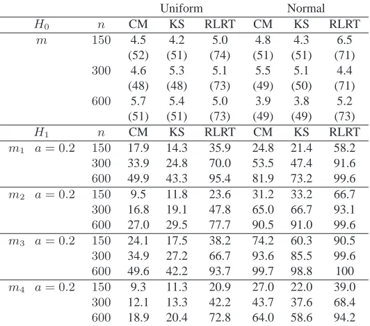
Fig. 1. CD4 count data. Observed individual profiles (gray lines) for patients treated with Zidovudine. The estimated function of the fixed effects using the local linear ker-nel estimator is shown by a dashed curve using a bandwidth of 8 weeks, and a cubic

parametric estimator is plotted by a solid curve.

From these plots it is difficult to extract any useful information, because the individual CD4

355

cell counts are quite noisy. However, the nonparametric estimator proposed in Section 2 is able

to capture the underlying structure in the data withp= 1. This local linear kernel estimator is

shown by the black solid curve in Figure 1. We have calculated this estimator by assuming model (2) with the response,Yij, being the CD4 cell counts, and with the covariate,Xij, being the time

in weeks. We chose a bandwidth of 8 weeks by eye. This choice considers the variability within

360

the data, and it is sufficient to provide a first visual impression about the underlying function. However, Gonz´alez-Manteiga et al. (2013) describe an automatic data-driven bandwidth selector for this type of kernel estimator.

To choose the covariance structure in model (2) we considered two candidates: a simple model

with only a random intercept, that is, withZij = 1; and a more complex model with both random 365

intercept and slope,Zij = (1, Xij)T. The second was used to calculate the local linear estimator

plotted in Figure 1. These models can be written in the forms (7) and (8), respectively. To decide which model is more appropriate, we calculated the AIC considering a quadratic polynomial for the function of the fixed effects. The AIC values are 27344 and 27359, suggesting that the model

with just a random intercept describes the random variations better. Therefore in the following 370

we work under model (7).

The local linear estimator in Figure 1 shows that the underlying time trend in the CD4 cell counts could be modelled by a quadratic or a cubic polynomial. However the impression from this graph depends on the degree of smoothness considered in the kernel estimator. We therefore

consider the tests proposed in this paper to decide between these two parametric models. First 375

we consider a quadratic polynomial as the null hypothesis. The resulting p-values are 1.2% using

Tn,KS, and 0.1% usingTn,CM. These statistics were calculated using the local linear estimator

and bandwidth parameter h=h0n−3/10, with h0 equal to the range of the covariate. With the

same type of kernel estimator and bandwidth choice, we now consider a cubic polynomial as

(13)

respectively. The tests confirm that the time trend in the CD4 cell counts, for the patients treated with Zidovudine, can be described by a cubic polynomial.

6. TESTING NONLINEAR FIXED EFFECTS ASSUMING A MORE GENERAL MODEL

We now consider a model motivated by a data application to growth studies with longitudinal

data. Our objective is to provide a suitable extension of the methods proposed in Sections 2 and 385

3. The data analysis itself and a brief simulation experiment show the practicability of the tests and their good performance in these settings. Further research is still necessary to derive the theoretical properties of the test under the new model.

Our motivating data are the orange tree dataset described by Draper & Smith (1998). The data

arise from an experiment in which trunk circumference in millimeter was measured for q = 5

390

orange trees on ni= 7 different occasions, over roughly a 4-year period of growth defined at

(xi1, . . . , xini) = (118,484,664,1004,1231,1372,1582) days for each tree. The interest in

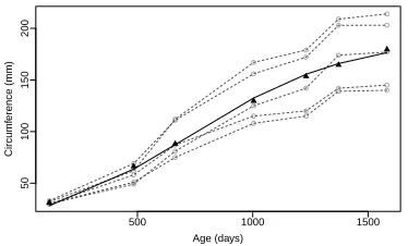
growth studies lies, among others, in characterizing the average growth pattern in the population. Thus testing whether a parametric function is appropriate for a particular growth study is of interest. Figure 2 shows the profile plot. Previous studies suggest that the marginal mean can be

395

described by a logistic model

E(Y |X) =β1[1 + exp{−(X−β2)/β3}]−1, (9)

which represents many common growth patterns (Draper & Smith, 1998). Neither the test of Pan & Lin (2005) nor that of Greven et al. (2008) can be used to check the suitability of this model, but our test can be easily extended to it.

400

The methods in Sections 2 and 3 were described under the semiparametric model (2), which assumes that the function of the random effects is linear, inducing the marginal covariance struc-ture given in (3). In order to apply the bootstrap method proposed in Section 3, the strucstruc-ture of the random effects needs to be specified. Serroyen et al. (2009) consider the mean structure model (9) for this dataset and suggest different models to describe the covariance structure. Among

405

several candidates, the following nonlinear mixed effects model, also suggested by Pinheiro & Bates (2000), provides a suitable representation of the underlying structure:

Yij = (β1+bi) [1 + exp{−(Xij −β2)/β3}]−1+ǫij. (10)

500 1000 1500

50

100

150

200

Age (days)

Circumf

[image:13.595.192.379.540.653.2]

erence (mm)

Fig. 2. Orange tree dataset. The dashed curves show the observed individual profiles. The parametric logistic esti-mator (solid curve) and the local linear estiesti-mator

(14)

Here, bi are independent and identically distributed normal variables with mean zero and

varianceτ2, andǫij are independent and identically distributed normal variables with mean zero

and varianceσ2₍_j _{= 1}_{, . . . , n}

i;i= 1, . . . , q). The marginal mean from this model is indeed the

410

logistic model (9), and it induces the covariance structure

Vi =var(Yi |Xi) =τ2sisTi +σ2Ini, (11)

withsi= ([1 + exp{−(Xi1−β2)/β3}]−1, . . . ,[1 + exp{−(Xini−β2)/β3}]

−1₎T_.

We propose the following extension of our model: 415

Yij =m(Xij) +viξ(Zij) +ǫij (j= 1, . . . , ni; i= 1, . . . , q), (12)

whereYij,Xij,Zij,mandǫij are specified exactly as before, but now the random effects

func-tionv_iξ(Zij)can be considered as a realization of a zero-mean nonlinear process depending on

a parameter vectorξ, with covariance functionγξ(Zij1, Zij2) =E{v

ξ

i(Zij1)v

ξ

i(Zij2)}. Assume also thatv_iξ(Zij)is independent ofǫij, conditionally onXij. The nonlinear mixed model defined

in (10) is a particular case of the semiparametric model (12), where m is the logistic func- 420

tion defined in (9),vξ_i(Zij) =bi[1 + exp{−(Xij −β2)/β3}]−1, and thebiare independent and

identically distributed normal variables with mean zero and varianceτ2.

Under model (12) our tests can be calculated in a straightforward way. The parametric and

nonparametric estimators ofmcan be derived using the three-step method of Section 2. Here it is

necessary to specify the marginal covarianceViinvolved in the global and local log-likelihoods, 425

(4) and (5), respectively. For the orange trees dataset we consider the structure Vi defined in

(11). Figure 2 shows two estimators ofm: the parametric logistic estimator and the local linear

estimator with bandwidthh= 500days. This figure suggests the adequacy of the logistic model.

To confirm this impression we perform the tests proposed in Section 3, and find that the

p-values for Tn,KS and Tn,CM are 58.7% and 55.7%, respectively. To derive these p-values we 430

have considered a modification of the bootstrap algorithm, given in the Supplementary Material. The finite sample performance of the tests described above is investigated in the Supplementary Material under a scenario which represents the performed data analysis.

ACKNOWLEDGEMENT

The authors thank Dr. S´anchez-Sellero for helpful discussions about computational issues, Dr. 435

Pan for supplying the AIDS dataset, and the Universidad de Granada for providing the com-puting time. This research was supported by the European Community’s Seventh Framework Programme, by the Spanish Ministry of Economy and Competitiveness and by the Belgian gov-ernment.

SUPPLEMENTARY MATERIAL 440

Supplementary Material available at Biometrika online includes the proofs of Proposition 1 and Theorems 1 and 2 in Section 3, and additional simulations and details for Sections 4 and 6.

REFERENCES

AKRITAS, M. G. & VANKEILEGOM, I. (2001). Non-parametric estimation of the residual distribution. Scand. J.

Stat. 28, 549–567. 445

(15)

GONZALEZ´ -MANTEIGA, W. & CRUJEIRAS, R. M. (2013). An updated review of goodness-of-fit tests for regression models. Test 22, 361–411.

GONZALEZ´ -MANTEIGA, W., LOMBARD´IA, M. J., MART´INEZ-MIRANDA, M. D. & SPERLICH, S. (2013). Kernel 450 smoothers and bootstrapping for semiparametric mixed effects models. J. Multivar. Anal. 114, 288–302.

GREVEN, S., CRAINICEAUNU, C., KUECHENHOFF, H. & PETERS, A. (2008). Restricted likelihood ratio testing for zero variance components in linear mixed models. J. Comp. Graph. Stat. 17, 870–891.

HENDERSON, D. J., CARROLL, R. J. & LI, Q. (2008). Nonparametric estimation and testing of fixed effects panel

data models. J. Econometrics 144, 257–275. 455

HUET, S. & KUHN, E. (2015). Goodness-of-fit test for Gaussian regression with block correlated errors. Statistics 49, 239–266.

LIANG, K. Y. & ZEGER, S. L. (1986). Longitudinal data analysis using generalized linear models. Biometrika 73, 13–22.

LIN, X. & CARROLL, R. J. (2000). Nonparametric function estimation for clustered data when predictor is measured 460 without/with error. J. Am. Statist. Assoc. 95, 520–534.

LIN, D. Y., WEI, L. J. & YING, Z. (2002). Model-checking techniques based on cumulative residuals. Biometrics 58, 1–12.

LOMBARD´IA, M. J. & SPERLICH, S. (2008). Semiparametric inference in generalized mixed effects models. J. R.

Statist. Soc. B 70, 913–930.

465

MEINTANIS, S. G. & PORTNOY, S. (2011). Specification tests in mixed effects models. J. Stat. Plan. Inference 141, 2545–2555.

NEUMEYER, N. & VANKEILEGOM, I. (2010). Estimating the error distribution in nonparametric multiple regression with applications to model testing. J. Multiv. Anal. 101, 1067–1078.

PAN, Z. & LIN, D. Y. (2005). Goodness-of-fit methods for generalized linear mixed models. Biometrics 61, 1000– 470

1009.

PARDO-FERNANDEZ´ , J. C., VANKEILEGOM, I. & GONZALEZ´ -MANTEIGA, W. (2007). Testing for the equality of

k_{regression curves. Stat. Sin. 17, 1115–1137.}

PARK, J. G. & WU, H. (2006). Backfitting and local likelihood methods for nonparametric mixed-effects models with longitudinal data. J. Stat. Plan. Inference 136, 3760–3782.

475

PEARSON, E. S. (1950). On questions raised by the combination of tests based on discontinuous distributions.

Biometrika 37, 383–398.

PINHEIRO, J. C. & BATES, D. M. (2000). Mixed-Effects Models in S and S-Plus, Springer, New York.

S ´ANCHEZ, B. N., HOUSEMAN, E. A. & RYAN, L. M. (2009). Residual-based diagnostic for structural equation models. Biometrics 65, 104–115.

480

SCHEIPL, F., GREVEN, S. & KUECHENHOFF, H. (2008). Size and power of tests for a zero random effect variance or polynomial regression in additive and linear mixed models. Comp. Stat. Dat. Anal. 52, 3283–3299.

SERROYEN, J., MOLENBERGHS, G., VERBEKE, G. & DAVIDIAN, M. (2009). Non-linear models for longitudinal data. Am. Stat. 63, 378–388.

SEVERINI, T. A. & STANISWALIS, J. G. (1994). Quasilikelihood estimation in semiparametric models. J. Am. 485

Statist. Assoc. 89, 501–511.

SPERLICH, S. & LOMBARD´IA, M. J. (2010). Local polynomial inference for small area statistics: estimation, vali-dation and prediction. J. Nonparametr. Stat. 22, 633–648.

VANKEILEGOM, I., GONZALEZ´ -MANTEIGA, W. & S ´ANCHEZ-SELLERO, C. (2008). Goodness-of-fit tests in para-metric regression based on the estimation of the error distribution. Test 17, 401–415. 490 WAND, M. P. & JONES, M. C. (1995). Kernel Smoothing. London: Chapman and Hall.

WOOD, S. N. (2013a). A simple test for random effects in regression models. Biometrika 100, 1005–1010. WOOD, S. N. (2013b). On p-values for smooth components of an extended generalized additive model. Biometrika

100, 221–228.

ZHANG, D. & LIN, X. (2003). Hypothesis testing in semiparametric additive mixed models. Biostatistics 4, 57–74. 495