Mass flow rate measurement of thermal creep flow from transitional to slip flow regime

Under consideration for publication in J. Fluid Mech.

Mass Flow Rate Measurement

of Thermal Creep Flow

from Transitional to Slip Flow Regime

Hiroki Yamaguchi

†

, Pierre Perrier

, Minh Tuan Ho

, J. Gilbert

M´

eolans

, Tomohide Niimi

, and Irina Graur

1

Dept. of Micro-Nano Systems Engineering, Nagoya University, Furo-cho, Chikusa, Nagoya, Aichi, 464-8603 Japan

2

Aix-Marseille Universit´e, CNRS, IUSTI UMR 7343, 5 rue Enrico Fermi, 13013 Marseille, France

3 _{James Weir Fluids Laboratory, Department of Mechanical and Aerospace Engineering,}

University of Strathclyde,

James Weir Building, 75 Montrose Street, Glasgow G1 1XJ, UK

(Received ?; revised ?; accepted ?.)

The measurements of the thermal creep flow through a single rectangular micro channel connected to two tanks maintained initially at the same pressure, but at different tem-peratures, is carried out for five noble gas species, in a large pressure variation range and for two temperature differences between the tanks. The time dependent pressure varia-tions in both cold and hot tanks are investigated, and the temperature driven (thermal creep) mass flow rate between two tanks is calculated from these data for the rarefaction parameter ranging from the transitional to slip flow regime. The measured mass flow rate is compared with the numerical solution of the S-model kinetic equation, showing good agreement with each other. A novel approximative expression to calculate the temper-ature driven mass flow rate in the transitional and slip flow regimes is proposed. This expression provides the results in good agreement with the measured values of the mass flow rate. In the slip flow regime, the thermal slip coefficient is calculated by employing the previously reported methodology, and the influence of the gas nature on this coeffi-cient is investigated. The measured values of the thermal slip coefficoeffi-cient agree well with the values available in the literature, indicating that this coefficient is independent of the shape of a channel.

1. Introduction

The thermal creep flow is one of the most interesting phenomena in the relatively high Knudsen number flows. This flow is induced by a temperature gradient along a surface, and it is directed from the cold to hot side. The Knudsen number, defined by the ratio of the molecular mean free path λto a characteristic length of a system Las Kn =λ/L, becomes large at a low pressure environment and/or in a small-scale flow field. Recently, it draws much attention due to the rapid development of the micro- and nano-technologies (Vargo et al. 1999; Passian et al. 2003; Young et al. 2003; Alexeenko et al. 2006; Han et al. 2007; Gupta & Gianchandani 2008; Sharipov 2011; Gupta et al. 2012; Martini et al. 2012; Dongari & Agrawal 2012; Graur & Ho 2014; Yamaguchi et al. 2014; Rojas-C´ardenas et al. 2015).

with the velocity slip boundary conditions are often employed (Kogan 1969; Cercignani 1990; Sharipov 2011). Two coefficients are usually involved in the expression of this velocity slip condition: the velocity slip and thermal slip coefficients. Among them, the thermal slip coefficient plays an important role in the thermal creep flow; therefore, we focus the present study on this coefficient.

The values of the thermal slip coefficient were derived theoretically from the kinetic theory of gases, using various kinetic equations (Boltzmann equation and model kinetic equations) and different models of the intermolecular potential, see review in Sharipov (2011). However, it is very important to improve our knowledge on the thermal slip coefficient and to obtain experimentally its values, especially because up to now only three works were devoted to the experimental extraction of this coefficient (Annis 1972; Porodnov et al. 1978; Rojas-C´ardenas et al. 2015). First, the thermal slip coefficient was extracted from the measurements of the thermomolecular pressure difference induced by the flow through a circular capillary, submitted to the large and small temperature gradient conditions in Annis (1972) and Porodnov et al. (1978), respectively. Recently, a novel procedure of the thermal slip coefficient extraction was proposed (Rojas-C´ardenas et al. 2015). The authors measured the stationary temperature driven mass flow rate through a micro tube of the circular cross-section to obtain then this coefficient. It is clear that with only these few experimental results, the information on the temperature driven flows and also on the thermal slip coefficient is not complete enough. Therefore, the new experimental data on the temperature driven gas mass flow rate are indispensable not only for the thermal management of the micro devices with the temperature gradients, but also for the extraction of the thermal slip coefficients for various gases.

In this study, we used our previously obtained (Yamaguchi et al. 2014) experimental data on pressure variation in time for the temperature driven gas flow through a rect-angular micro channel to obtain new reliable characteristics on the thermal creep flow. The experimental values of the thermal slip coefficient are provided for five noble gases (Helium, Neon, Argon, Krypton, Xenon) and the influence of the gas nature on this co-efficient is studied. Moreover, a novel procedure to obtain the temperature driven mass flow rate in the transitional flow regime, useful in many rarefied flows applications, is proposed. The experimental data are analyzed to characterize the thermal creep flows in wide flow regimes ranging from the transitional to slip flow regime.

2. Experimental data analysis

The details and sketch of the experimental apparatus used in present work can be found in Yamaguchi et al. (2014). The rectangular micro channel made of PEEK with the height of H = 0.22±0.01mm, the width of W = 6mm, and the length of L = 73mm was employed. The temperature gradient along the micro channel was realized by two blocks with gas reservoirs inside placed at both ends of the micro channel, whose temperatures were controlled by an electrical heater for the hot side and a circulating water for the cold side, respectively. The temperature of each block was monitored by a K-type thermocouple (TC) placed on the outside of the blocks. Temperature for the hot reservoirTHand that for the cold reservoirTCwere maintained to realize two cases of the temperature difference ∆T : 1)TH= 347.1±0.5K,TC= 289.2±0.2K, where ∆T = 57.9K and 2)TH= 337.0±0.6K,TC= 299.6±0.4K, where ∆T = 37.4K. The both temperature differences were chosen to have the same mean temperature Tm = (TC+TH)/2 for two cases asTm= 318K. Here, twice of the standard deviation (2σ) was used as an uncertainty of the temperature conditions.

forming a circuit with insertion of a micro valve (Parker Hannifin). When the micro valve is open, there is the stationary thermal creep flow through the micro channel from the cold to hot sides; while the flow through the large diameter tube maintains pressures equally at both reservoirs by compensating the thermal creep. By closing the micro valve, the flow in the large diameter tube is blocked, and there is only the thermal creep flow inside the micro channel. With time evolution, the pressure difference occurs between the cold and hot reservoirs as a result of the thermal creep flow, inducing a pressure driven flow in the opposite direction to the thermal creep flow. The pressure variations with time in two reservoirs are well fitted by the exponential functions (Yamaguchi et al. 2014; Rojas-C´ardenas et al. 2011, 2013) as,

pC(t) =pi− |pC,∞−pi|

(

1−e−t/τC )

, pH(t) =pi+|pH,∞−pi|

(

1−e−t/τH )

, (2.1)

wherepC(t) and pH(t) are the pressure variation in time in the cold and hot reservoirs, respectively, t is a time, pi is the initial pressure, which was common for the hot and cold reservoirs, pC,∞ and pH,∞ are the final equilibrium pressures in the cold and hot reservoirs, respectively, andτCandτHare the relaxation times, at the cold and hot parts, respectively. The pressures in two reservoirs were measured by capacitance diaphragm gauges (CDGs) (Inficon CDG045D (hot side), CDG025 (cold side)); but there were tem-perature differences between reservoirs and CDGs, resulting, in the both cold and hot sides, in pressure differences between a reservoir and a CDG due to the thermal creep flow along the CDG tube. Therefore, the pressure was corrected by using the Takaishi & Sensui formula (Takaishi & Sensui 1963).

The timet= 0 was determined as the closing moment of the micro valve, which was decided by monitoring an applied voltage to the micro valve. Since the stationary thermal creep flow was not yet disturbed att= 0, the mass flow rate of the thermal creep flow is obtained from the measured time variation of pressures as,

˙

M = V

RT dp(t)

dt

t=0

, (2.2)

whereV,T,p(t) are the volume, the temperature, and pressure of a reservoir, respectively, andRis the specific gas constant. The pressure variation ratedp/dt|_t=0was calculated by differentiating the fitted exponential functions (Eq. (2.1)). The stationary mass flow rate can be calculated for each of the cold and hot reservoirs, which should be equal from the mass conservation. In this study, the mass flow rate of the cold reservoir, calculated from pC(t), is used, because there is a slight delay at the starting of the pressure variation in the hot reservoir. The reason of the delay might be the fact that the temperature difference was quite large between the hot reservoir (74 ◦C or 64 ◦C) and the internal temperature of the pressure gauge (45◦C), where a thermal creep flow was induced and it could affect the pressure measurement.

To analyze the time dependent characteristics of the thermal creep flow, namely the mass flow rate, the rarefaction parameter is used

δ= pH

µ√2RT, (2.3)

assumed to have the power law dependence on temperature,

µ=µref

( T Tref

)ω

, (2.4)

where µref is the viscosity coefficient at the temperature Tref and ω is the viscosity index (Bird 1994). The rarefaction parameter is defined by Eq. (2.3) as a local value, depending on the local values of pressure and temperature, which were, however, not measured. Therefore, the mean rarefaction parameter δm was calculated by using the mean temperatureTmand the initial pressure pi as,

δm=

piH

µ(Tm)√2RTm

. (2.5)

The initial pressurepi was varied from 66 Pa to 1270 Pa for every gas species, and the mean rarefaction parameterδmin the range between 0.6 to 40 were employed. Therefore, the flow was ranged from the transitional to slip flow regime.

3. Numerical simulations to estimate the mass flow rate inside the

channel

3.1. Numerical mass flow rate

The detailed information about the local flow characteristics inside the channel is impor-tant for the analysis of the average characteristic measurements, as the mass flow rate; however, it was not easy to obtain them experimentally. Therefore, we also employed a numerical simulation for the further analysis.

Various authors have analyzed stationary thermal creep flows through rectangular cross-section channels or parallel plates by using the linearized kinetic models (BGK (Stvorik et al. 1978) and S-model (Sharipov 1999; Graur & Ho 2014)) or by solving the linearized Boltzmann equation (Ohwada et al. 1989; Sone 2002). These approaches are indispensables in the transitional flow regime, where the continuum approach does not valid anymore, but the collisionless Boltzmann equation cannot be applied yet. In all these publications, it was assumed that the local pressure and temperature gradients along the channel

H p

dp dz 1,

H T

dT

dz 1, (3.1)

were small enough for the linearization of the kinetic equations. This assumption, Eq. (3.1), allows the presentation of the mass flow rate through a rectangular cross-section channel in the linear form

˙

M =√HW p

2RT (

−Gp(δ, α)H p

dp

dz +GT(δ, α) H T

dT dz

)

. (3.2)

In expressions (3.1) and (3.2), thez-axis coincides with the direction of the temperature gradient and of the channel’s largest dimension (channel lengthL). The local dimension-less flow rates,GpandGT, are induced by the local gradients of pressure and temperature, Eqs. (3.1), respectively, and they depend on the local rarefaction parameterδand on the accommodation coefficientα. In the numerical simulation we assumed, unless otherwise stated, the full accommodation,i.e.α= 1, at walls in the frame of the Maxwell diffuse-specular kernel. It is important to note that T and p in Eq. (3.2) are the temperature and pressure at a local point inside the channel, respectively.

and the values of the dimensionless mass flow ratesGp(δ) andGT(δ), obtained in Graur & Ho (2014) for the channel withW/H ratio equals to 0.0367, which corresponds to the real channel’s dimensions. The equality of the pressure in both inlet and outlet reservoirs was used as the boundary conditions for the pressure. From this integration, the mass flow rate

˙

M was obtained together with the pressure distribution along the channel, see Sharipov (1999); Graur & Ho (2014) for more details. To extract these both flow characteristics, a linear temperature distribution along the channel walls was assumed. In Section 4.1, the numerical results will be compared with the mass flow rate measurements.

3.2. Effect of pressure profiles inside the micro channel

The mass flow rate ˙M, expressed at a local point is, as mentioned above, known to be decomposed into two terms, as in Eq. (3.2). The first and second terms represent the pressure and temperature driven flows, respectively. Even though the flow inside the micro channel at t = 0 was largely dominated by the temperature driven flow (Rojas-C´ardenas et al. 2013), there would be a slight pressure gradient along the micro channel, which would induce a flow. The fraction of this flow rate, caused by the pressure gradient, can be estimated from the first term of Eq. (3.2),i.e.the reduced flow rate induced by a pressure gradient. To obtain this information on the part of the pressure gradient induced mass flow rate in the total mass flow rate, Eq.(3.2) was integrated along the channel as following,

˙

M =−1

L ∫ pH

pC

H2_{W p}

√

2RTGp(δ) dp

p +

1 L

∫ TH

TC

H2_{W p}

√

2RTGT(δ) dT

T (3.3)

=−M˙p+ ˙MT. (3.4)

To establish Eq. (3.3) from Eq. (3.2), the mass conservation property was used. When integrating the first term in Eq. (3.3), we implemented the pressure distribution along the channel, obtained, as it was explained in Section 3.1, from the numerical solution of Eq.(3.2). For the integration of the second term in Eq. (3.3), the linear distribution of the temperature was assumed. After integration, the ratio of pressure driven mass flow rate,M˙p, to the whole mass flow rate ˙M was calculated. It was found that the termM˙p was appeared to be less than 0.1% of the full mass flow rate ˙M for ∆T = 37K and less than 0.2% for ∆T = 58K, respectively. These results indicate that the pressure profile along the micro channel is nearly flat,i.e.the pressure driven flow is negligible att= 0, when the mass flow rate is driven only by the temperature gradient.

3.3. Temperature driven mass flow rate

Taking into account the previous results, obtained in Section 3.2, on the part of the pressure induced mass flow rate in the total mass flow rate, it is reasonable to approximate the total mass flow rate, Eq.(3.3), only by the temperature gradient term:

˙

M 'M˙T=

1 L

∫ TH

TC

H2_{W p}

√

2RTGT(δ) dT

T . (3.5)

pi in Eq. (3.5), then, after integration of Eq. (3.5), the thermal creep mass flow rate becomes

˙

MT'M˙TA=GT(δm)

2H2W

L pi

(

1

√

2RTC

−√ 1

2RTH

)

. (3.6)

To validate the two approximations: GT(δ) by GT(δm) and the local pressure by its initial valuepi, when expression (3.6) was obtained, the comparison with the originally simulated mass flow rate M˙, deduced from Eq. (3.3), see Section 3, was carried out. The discrepancies (

(

˙

M_TA−M˙

)

/M˙) appeared to be less than 0.7% for the whole range of the flow regime,δm = [0.5,40]. Thus, it is reasonable to estimate that the variation ofGT as a function of δ was very small along the channel and that theGT(δ) value is well represented by GT(δm), as well as to estimate the pressure along the channel by the initial pressurepi. The proposed expression, Eq. (3.6), is directly compared with the measured mass flow rate in Section 4.3.

Expression (3.6) can be also easily modified to show the dependency of the mass flow rate on the gas viscosity

˙

MT'M˙

µ

T=µ(Tm)GT(δm) 2HW

L δm

(√

Tm

TC

− √

Tm

TH

)

. (3.7)

This last expression will be used in Section 4.1 to analyze the experimental data on the mass flow rate as a function of the mean rarefaction parameterδm.

4. Experimental mass flow rate.

The experimental mass flow rates were obtained from the pressure variation rate at t= 0 in the cold reservoir, according to Eq. (2.2), for various values of the initial pressure and, therefore, for various values of the mean rarefaction parameter, Eq. (2.5).

4.1. Comparison with numerical results

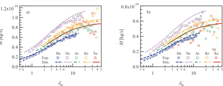
The experimental and numerical results of the mass flow rate ˙M are compared in Fig. 1 for the two values of the temperature difference ∆T between the reservoirs. The lines from the numerical simulation, considering the full accommodation at walls and the linear temperature distribution, show good agreements with the plots of the experimental results for the whole range of the experimental conditions, i.e.from the transitional to slip flow regime 0.5< δm<40. With increase inδm, the mass flow rate increases in the transitional flow regime and approaches asymptotically to a constant value in the slip flow regime. The measured results are slightly scattered in the large rarefaction parameter region, which could be caused by very small pressure variations |p_∞−pi| in Eq. (2.1) for both the cold and hot reservoirs due to the weak thermal creep flow, resulting in less accurate measurements of the pressure variation rates.

Let us now analyze the influence of the gas viscosity on the mass flow rate. Expression (3.7) for the temperature driven mass flow rate as a function ofδmis directly proportional to the viscosity coefficient. Furthermore, because the dimensionless mass flow rate GT, is nearly independent of gas species for noble gases (Sharipov & Bertoldo 2009), then Eq.(3.7) predicts that the mass flow rate is nearly proportional to the viscosity coefficient for a given value ofδm. More precisely, the viscosity coefficients at the mean temperature Tm, calculated from Eq. (2.4), are equal to 2.06, 3.29, 2.39, 2.63 and 2.40×10−5_{Pa·s for} Helium, Neon, Argon, Krypton and Xenon, respectively. As it can be observed in Fig. 1, the mass flow rates are shown to be nearly proportional to the viscosity coefficients, listed above.

Moreover, it is interesting to note that the mass flow rates for Argon and Xenon show quite similar values, when the mass flow rate ˙M is plotted as a function of δm, see Fig. 1. Indeed these gas species have similar values ofµref (Argon 2.117·10−5kg/(s·m) and Xenon 2.107·10−5_{kg/(s·m)) and ω (Argon 0.81 and Xenon 0.85) resulting in similar} value not only forµ(Tm) but forµat every temperature. Consequently, from the previous comments, we can predict for the mass flow rate of these gas species the similar values at the same δm, verified in Fig. 1. Let us note that, experimentally, the same δm is ob-tained for two gases by choosing the respective pressures such aspAr/pXe=

√

mXe/mAr,

following Eq.(2.5).

4.2. Influence of gas-surface interaction and temperature profile

In the numerical simulation, the full accommodation of the molecules at the wall and the linear temperature profile were assumed. However, the incomplete accommodation is often reported even for machined surfaces (Yamaguchi et al. 2012; Hadj Nacer et al. 2014) and the low heat conductivity of the channel’s material might result in a non-linear temperature profile (Rojas-C´ardenas et al. 2015). To verify the relevance of these two assumptions, the effects of an incomplete accommodation and of a temperature profile shape, were examined numerically.

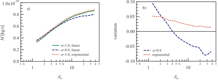
From the numerical results, we obtained that the incomplete accommodation influences essentially the mass flow rate. Ifα= 0.8, which is close to the value in Rojas-C´ardenas et al. (2015), the mass flow rate increases, compared to its value for the complete ac-commodationα= 1, by at most 17.8% with Helium at the lowestδ. But whenδ&4, it decreases compared to its value forα= 1 and reaches−7.9% atδ∼27.5. For the other gases, the tendency is similar, but the deviation extent in the mass flow rate compared to its value forα= 1 is smaller than the case for Helium. It was also found that the mass flow rate decreasing due to the incomplete accommodation is independent of the applied temperature difference.

!"# $% $ !$ $!& $!' $!( $!" $!$ !)))))))))) )*+,-./

0 ' " 1 ( 0 '

$ " 1 ( 0 d2

)))))))))))))))34)))))54)))))67))))))87)))))94)) :#;!))))) ) ) ) ) <=2!)))))) ) ) ) )

>? !"#$

%$

!&

!'

!(

! !)))))))))) )*+,-./

0 &

$ ( 1 ' 0 & $ ( 1 ' 0 d2

)))))))))))))))34)))))54)))))67))))))87)))))94)) :#;!))))) ) ) ) ) <=2!)))))) ) ) ) )

>?

Figure 1.The experimental mass flow rate ˙M were compared with the values obtained from the numerical simulations. a) is for ∆T = 58K and b) is for ∆T = 37K. The symbols rep-resent the experimental results of 5 (blue) Helium, 2 (purple) Neon, (green) Argon, 3 (orange) Krypton, and4(red) Xenon, respectively. The results of the simulation considering the full accommodation at walls plotted by a dashed line for Helium, a dotted line for Neon, a dashed-dotted line for Argon, a dashed-two dotted line for Krypton, and a solid line for Xenon, respectively. The maximums of the vertical axes are set in the same ratio as ∆T for a):b).

flow rate, while the incomplete accommodation decreases it for the higher gas rarefaction (lowδ) and decreases for high values of δ. To see the tendency above more clearly, the two deviations in the mass flow rate were also plotted in Fig. 2 b). The first deviation

(

˙

M(α= 0.8)−M˙(α= 1)

)

/M˙(α= 1) shows the influence of the incomplete accommo-dation of the molecules with the channels’ wall, which leads to increase of the mass flow rate compared to the mass flow rate for α = 1 for the small delta and decrease with the highδ, see Fig. 2 b). The deviation of the mass flow rate due to the change in the shape of the wall temperature profile

(

˙

M(Texp−M˙(Tlin))

)

/M˙(Tlin) is positive for all δ. As it can be seen from Fig. 2 b), the two effects of the incomplete accommodation and of the temperature profile shape compensate each other in the consideredδm range [3,40]. Probably, this is a reason why the numerical estimation gives good agreement with the experimental data, see Fig. 1, even though ideal conditions were assumed in the simulations. This agreement could be resulted from the two realistic effects of the incom-plete accommodation and non-linear temperature profile varying the mass flow rate in opposite directions.

4.3. Reduced mass flow rate GT

Simple explicit expression for the temperature driven mass flow rate is obtained in Sec-tion 3.3, Eq.(3.6). However, this expression (3.6) involves the numerical results on GT coefficient. As it was mentioned above, this coefficient was calculated numerically by various authors. Therefore, we can derive the expression ofGT from our experimental results and compare with the available results of the numerical simulations.

!"# "$ "

"!%

"!&

"!'

"!(

"!" !)))))))))) )*+,-./

0 & ( 1 ' 0 &

" ( 1 ' 0 d2

)a3 !"4)56789: )a3"!%4)56789: )a3 !"4)8#;<787=695

9>

!"#! !"!$ !"!! !"!$ !"#!

%&'(&)(*+

$ ,

# - . / $ , #! - . / $ d0

1a2!"3 1456*+4+)(&7

89

Figure 2.The effects of the incomplete accommodation and temperature profile are evaluated by the numerical simulations. In a), the mass flow rate of the original full accommodation of the molecules at the wall and the linear temperature profile (green solid line) is plotted with those of the incomplete accommodation and the linear temperature profile (blue dashed line); and of the complete accommodation and the exponential temperature profile (red dotted line); all results for Argon as a typical example. In b), the variations which are the differences for two effects from the original divided by the original mass flow rate are plotted. The vertical axis in (a) is modified from Fig. 1.

flow rateGTmight be considered as independent of gas species at least for noble gases. The reduced flow ratesGT of helium, neon and argon for ∆T = 58K is listed with the measured mass flow rates in Table 1.

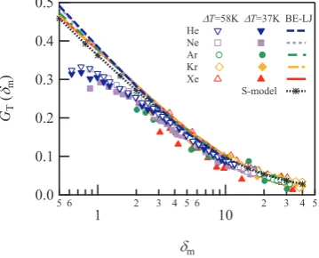
Until the slip flow regime, the obtained experimental results show good agreement with the numerical results. However, a small discrepancy appears in the near free molecular regime, i.e.in the small δ region. It seems very difficult to explain this discrepancy as resulting from an incomplete accommodation at the surface. As it was shown in the numerical simulations (Loyalka 1975; Loyalka & Hickey 1991; Sharipov & Seleznev 1998) and through presented here results, an incomplete accommodation would lead to an increase in the reduced flow rate GT in the small δ region, and it is not consistent with the results in Fig. 3. Another possibility is the measurement errors increase with decreasing in δ, because the measurements are quite difficult in the free molecular flow regime.

5. The slip flow regime: the thermal slip coefficient

σ

5.1. Extraction of the thermal slip coefficient from the mass flow rate

In the previous section, it was shown that in the transitional and slip flow regimes the measured thermal creep mass flow rate is in very good agreement with the numerical re-sults. However, the mass flow rate can be obtained only numerically through the solution of the kinetic equation. From the previous study (Yamaguchi et al. 2014), it was shown that the thermal creep phenomenon is also important in the slip flow regime. Therefore, it will be worth to have an analytical solution in the slip flow regime (Rojas-C´ardenas et al. 2015).

!"

!#

!$

!%

!&

!

'

()d*

+

" ,

& % $ # " , & % $ # " d*

((((((D!-"./((D!-$0/((12345( 67((( (((((((( ((((( 87((( (((((((( ((((( 9:(((( (((((((( ((((( /:(((( (((((((( ((((( ;7((( (((((((( ((((( (((((((((((((((((((((<3*=>7?((( ( (

Figure 3.The reduced flow rateGTobtained from the experimental results are plotted for both

∆T = 58K and ∆T= 37K. The symbols represent the experimental results for ∆T = 58K of5 Helium,2Neon,Argon,3Krypton, and4Xenon, respectively. The data for ∆T = 37K are plotted with filled markers. The numerical results for the rectangular channel (H/W= 0.0367) for the full accommodation, obtained by the S-model kinetic simulation in (Graur & Ho 2014), are plotted by a dotted line with markers. The numerical results for the flow between two parallel plates with the full accommodation and for Lennard-Jones intermolecular potential in (Sharipov & Bertoldo 2009) forδm <10 are also plotted by a dashed line for Helium, a dotted line for

Neon, a dashed-dotted line for Argon, a dashed-two dotted line for Krypton, and a solid line for Xenon, respectively.

mass flow rate is calculated; thus, the equation has the form ∂2_u

z

∂x2 +

∂2_u z

∂y2 = 0, (5.1)

where z-axis coincides with the direction of the temperature gradient and the thermal creep flow is induced in thezdirection with the velocityuz. The thermal slip boundary condition on a flat wall has the form

uz|wall=σT µ ρT

dT

dz, (5.2)

where ρ is the gas density. The solution of the Stokes equation, Eq. (5.1), with the thermal slip boundary condition, Eq. (5.2), is a constant velocity over the whole cross section (Sharipov 2011). Thus, the mass flow rate is obtained as,

˙

M =σTHW

µ T

dT

dz. (5.3)

By using Eq. (2.4) for the viscosity coefficient, the mass flow rate is expressed as, ˙

M =σT

HW µref

Tω

ref

F, (5.4)

whereF =Tω−1dT /dz, and onlyF varies by local conditions. As it was pointed out in Section 4.1, in this study the temperature profile along the channel was not measured; therefore, the mean value of F was calculated by integrating its expression along the channel:

F = 1 L

∫ TH

TC

Tω−1dT = T

ω H −T

ω C

ωL , (5.5)

Table 1.The measured mass flow rates ˙M[×10−10kg/s] and reduced flow ratesGTof typical

gas species for ∆T= 58K.

He Ne Ar

δm M˙ GT δm M˙ GT δm M˙ GT

0.624 0.137 0.324 0.873 0.307 0.326 1.70 0.355 0.264 0.739 0.167 0.333 1.05 0.349 0.306 2.01 0.409 0.256 0.865 0.193 0.328 1.22 0.399 0.303 2.36 0.430 0.231 0.998 0.214 0.316 1.41 0.435 0.285 2.70 0.487 0.228 1.11 0.233 0.308 1.58 0.469 0.274 3.03 0.496 0.206 1.24 0.249 0.294 1.75 0.511 0.270 3.38 0.531 0.199 1.48 0.278 0.276 2.10 0.571 0.251 4.01 0.554 0.175 1.73 0.313 0.266 2.44 0.611 0.232 4.73 0.636 0.169 1.98 0.341 0.253 2.78 0.629 0.209 5.37 0.655 0.153 2.22 0.363 0.239 3.14 0.708 0.208 6.04 0.611 0.127 2.47 0.402 0.239 3.48 0.718 0.190 6.72 0.670 0.125 2.72 0.418 0.225 3.83 0.756 0.182 7.41 0.702 0.119 2.98 0.429 0.210 4.18 0.795 0.175 8.08 0.651 0.102 3.22 0.448 0.204 4.52 0.796 0.162 8.75 0.739 0.106 3.47 0.465 0.196 4.87 0.819 0.154 9.41 0.741 0.0989 3.71 0.476 0.188 5.24 0.845 0.148 10.1 0.700 0.0874 4.33 0.526 0.178 6.09 0.886 0.134 11.7 0.697 0.0751 4.94 0.526 0.156 6.94 0.896 0.119 13.4 0.746 0.0698 5.57 0.532 0.140 7.83 0.920 0.108 15.1 0.787 0.0654 6.19 0.560 0.132 8.70 0.939 0.099 16.8 0.855 0.0638 6.80 0.607 0.130 9.55 0.928 0.089 18.5 0.787 0.0533 7.41 0.587 0.115 10.4 0.997 0.087 20.2 0.798 0.0496 8.04 0.587 0.107 11.3 0.954 0.077 21.8 0.787 0.0453 8.67 0.592 0.0996 12.2 0.965 0.072 23.6 0.737 0.0393 9.28 0.629 0.0987 13.1 1.03 0.072 25.2 0.758 0.0377 9.90 0.624 0.0918 13.9 1.04 0.069 26.9 0.829 0.0388 10.5 0.629 0.0871 14.8 0.956 0.059 28.6 0.736 0.0323 11.1 0.613 0.0803 15.7 1.07 0.062 30.3 0.842 0.0349 11.7 0.646 0.0800 16.5 1.02 0.056 31.9 0.710 0.0279

The thermal slip coefficient σT was calculated from the measured mass flow rate by using the analytical expression for the thermal creep mass flow rate, Eqs. (5.4) and (5.5):

σT= ˙M /M˙ref, M˙ref=

HW µref

Tω

ref

T_Hω−T_Cω

ωL . (5.6)

!"

!#

#!"

#!# s$

"# %# &# '# # #

d( )))))))))))))))))*+))))),+)))))-.)))))/.)))))0+ D 1"2/) ) ) ) ) D 1&3/) ) ) ) ) -4+.56+)) ) ) ) )

Figure 4.The thermal slip coefficientsσT obtained from the experimental results are plotted

for ∆T = 58K and ∆T = 37K. They are plotted againstδm, validating that the coefficient is

independent ofδm. The symbols represent the experimental results for ∆T= 58K of5Helium, 2Neon,Argon,3Krypton, and4Xenon, respectively. The data for ∆T= 37K are plotted with filled markers. The averaged values over both two ∆T cases are plotted by a dashed line for Helium, a dotted line for Neon, a dashed-dotted line for Argon, a dashed-two dotted line for Krypton, and a solid line for Xenon, respectively.

Table 2.Obtained thermal slip coefficients from the averaged mass flow rate over the range of δm= [10,40]. The errors are 95% confidence interval of the fitting procedure.

all ∆T = 58K ∆T = 37K

He 0.916±0.018 0.921±0.171 0.911±0.030 Ne 0.912±0.033 0.929±0.035 0.895±0.065 Ar 0.957±0.057 0.971±0.038 0.944±0.116 Kr 1.000±0.052 1.039±0.082 0.961±0.070 Xe 1.029±0.078 1.074±0.082 0.983±0.142

very small and within the errors interval. It is important to note that the number of the data in the range, used for the averaging, was different for every gas species, since the rarefaction parameterδ, Eq. (2.3), is different between gas species at the same pressure condition due to the difference in the molecular weights.

5.2. Extraction of σTby asymptotic expression for the mass flow rate

The above mentioned mass flow rate, obtained by solving the Stokes equation with ther-mal slip boundary condition, is a first order solution. The higher order solution for the dimensionless temperature driven mass flow rateGTwas obtained from the kinetic the-ory in form of an asymptotic expression in Loyalka & Hickey (1989) and in term of the dimensional mass flow rate, it reads

˙

M = HW µ

T dT

dz [

AT+B

T

δ +O

(

1 δ2

)]

, (5.7)

comparing Eqs. (5.3) and (5.7), it is clear that the both expressions are similar andAT can be identified to the thermal slip coefficientσT in the slip flow regime. However, the asymptotic expression, Eq.(5.7), contains the additional term of the order ofO(1/δ) and therefore allows to determineσT coefficient more accurately. As in the case with the first order extraction, expression (5.7) was integrated along the channel by using the mass conservation property. To integrate expression (5.7), the rarefaction parameterδwas also related to the mean rarefaction parameter δm and the local temperature and pressure values, see Rojas-C´ardenas et al. (2015) for more details. Finally, the expression of the mass flow rate through mean and reservoirs’ values is obtained

˙

M = ˙Mref

[

AT+B

T_B 2

δm

+O (

1 δ2 m

)] ,

B2=

T_H2ω+1/2−T_C2ω+1/2 (2ω+ 1/2)Tmω+1/2

ω

Tω

H−TCω

. (5.8)

The previous expression, by analogy with Eq. (5.6), can be rewritten in the following form

G(δm) = ˙M /M˙ref =AF+

BFB2

δm

. (5.9)

It is clear that the measured mass flow rate can be fitted in form of Eq. (5.9) and the fitting coefficientAFcan be associated with the coefficientσT.

Since the asymptotic expression allowed to enlarge the applicable flow regime to the transitional flow regime, the measured mass flow rate in the range ofδm = [3,40] was employed for the fitting procedure. The experimental data with the fitting curves are plotted in Fig. 5. The coefficientsAF and BF, obtained from the fitting of the experi-mental data according to Eq. (5.9) are listed in Table 3. The coefficient B2 was quite close to unity and the largest deviation from unity was less than 0.1%. Therefore, to calculate the thermal slip coefficients from all the data for both ∆T = 58K and 37K, B2 = 1 was assumed. The errors from B2 in the calculation of the coefficientBF was also neglected, since the values were almost constant and the errors in the temperature measurement should be very small.

These results are theoretically much reliable compared to the first order extraction in Table 2, because a greater number of data were employed for the fitting procedure, which is especially true for Helium. In addition, the values are quantitatively in quite good agreement with the numerical (Sharipov & Bertoldo 2009) and the experimental results in the literature (Annis 1972; Porodnov et al. 1978; Rojas-C´ardenas et al. 2015). This agreement indicates notably that the thermal slip coefficient is independent of the cross-sectional shape of the channel.

Comparing between gas species, the thermal slip coefficient increases with an increase in the molecular weight, except Neon. Neon gives a little smaller value compared with Helium. It shows the same tendency with the case of the first order extraction, see Table 2. This tendency is exactly the same with the numerical results (Sharipov 2011) and with the experimental values obtained previously in Annis (1972); Porodnov et al. (1978).

!"

!#

#!"

#!#

$

%&d'

(

) * " + , - .

# / ) * " d'

%%%%%%%%%%%%%%%%%01%%%%%21%%%%%34%%%%%%54%%%%%61 D 7"-5% % % % % D 7),5% % % % % 89::1;%%%%%% % % % %

Figure 5.FunctionG(δm), Eq. (5.9), as a function ofδm, obtained from the experimental results

are plotted for ∆T = 58K and ∆T = 37K. The symbols represent the experimental results for ∆T = 58K of5 Helium,2Neon,Argon,3Krypton, and4Xenon, respectively. The data for ∆T = 37K are plotted with filled markers. The fitting curves over both two ∆T cases are plotted by a dashed line for Helium, a dotted line for Neon, a dashed-dotted line for Argon, a dashed-two dotted line for Krypton, and a solid line for Xenon, respectively.

Table 3.Obtained thermal slip coefficients AF andBF by the fitting of the asymptotic mass flow rate expression over the range ofδm= [3,40].B2was assumed to be unity in the calculation

for “all”. The errors are 95% confidence interval of the fitting procedure, and uncertainties from B2 are neglected.

all ∆T = 58K ∆T= 37K

AF BF AF BF AF BF

He 1.006±0.020 −1.147±0.113 1.026±0.027 −1.196±0.149 0.985±0.023 −1.100±0.127 Ne 0.998±0.029 −1.226±0.172 1.013±0.025 −1.197±0.147 0.983±0.049 −1.255±0.290 Ar 1.017±0.057 −1.274±0.406 1.038±0.035 −1.248±0.249 0.997±0.105 −1.299±0.763 Kr 1.061±0.053 −1.327±0.400 1.111±0.076 −1.442±0.566 1.012±0.074 −1.212±0.554 Xe 1.102±0.085 −1.746±0.626 1.142±0.087 −1.547±0.640 1.061±0.142 −1.946±1.050

It would be also interesting to calculate the accommodation coefficient from the ob-tained experimentally thermal slip coefficient, by using, for example, the following expres-sion proposed in (Sharipov 2011) in the frame of the Maxwell diffuse-specular boundary condition and using the S-model kinetic equation

σT= 0.75(1 + 0.5α). (5.10)

equation with the HS potential varies from 3% for α= 0 to 12% for α= 1 (Sharipov 2011).

Moreover, when one extracts an experimental value of the accommodation coefficient from the thermal slip coefficient by using Eq. (5.10), it is clear that the uncertainties onαrepresents 8/3 of the uncertainties on σTand so would lie beyond the acceptable accuracy, especially for Argon and Xenon. In addition, taking into account this large difference in numerical values of σT described above, the implementation of Eq. (5.10) itself to extract the value of the accommodation coefficient can engender a large additional error. Therefore, it is not reasonable to calculate the accommodation coefficient from the experimental results in this study. Nonetheless, the accommodation coefficient which corresponds to the obtained thermal slip coefficient would be not so far from unity, which is in consistence with the above mentioned characteristics from theBT _coefficient.

6. Conclusion

The thermal slip coefficient in the slip flow regime and the reduced flow rate in the transitional flow regime were obtained for five noble gases in the rectangular cross section geometry from the experimental measurement of a pure thermal creep flow.

The mass flow rate was compared with the numerical result by solving the S-model kinetic equations, showing good agreement for all cases in all flow conditions. Then, the numerical simulation was employed to validate the assumptions for involved methodology. The reduced flow rate GT was directly calculated from the experimentally measured mass flow rate by assuming the negligible variation in pressure and the rarefaction pa-rameterδ in the micro channel. The obtained values showed good agreement with the numerical results.

The thermal slip coefficientσT of five noble gases was affected by gas species and it increases with increasing in the molecular weight, except Neon. Neon showed slightly smaller value than the result of Helium. Analyzing the influence of the channel geometry, it was found that theσT coefficient of the rectangular channel showed quite close value to that of the circular tube, indicating the value is independent of the cross-sectional shape of the channel.

Acknowledgments

The micro channel and the blocks were fabricated at Institute for Micro Process En-gineering (IMVT), Karlsruhe Institute of Technology (KIT) in the framework of the European Community’s Seventh Framework Program (FP7/2007-203 under grant agree-ment n 215504). This study was partially supported by the Overseas Visits Program for Young Researchers by Nagoya University Venture Business Laboratory and the program “Creation of Materials, Processes and Systems Provided with New and High Functional-ity” in the fund “Institutional Program for Young Researcher Overseas Visit” sponsored by JSPS. This work has been carried out in the framework of the Labex MEC (ANR-10-LABX-0092) and of the A*MIDEX project (ANR-11-IDEX-0001-02), funded by the ”Investissements d’Avenir” French Government program managed by the French Na-tional Research Agency (ANR).

REFERENCES

mod-eling of temperature driven flows in short microchannels. International Journal of Thermal Sciences45(11), 1045–1051.

Annis, B. K.1972 Thermal creep in gases. Journal of Chemical Physics57(7), 2898–2905.

Bird, G. A. 1994 Molecular Gas Dynamics and the Direct Simulation of Gas Flows. Oxford Science Publications, Oxford University Press Inc., New York.

Cercignani, C.1990 Mathematical methods in kinetic theory. Plenum Press New York Press, New York, London.

Dongari, N. & Agrawal, A. 2012 Modeling of navier-stokes equations for high knudsen

number gas flows. International Journal of Heat and Mass Transfer55, 4352–4358.

Graur, I. & Ho, M. T.2014 Rarefied gas flow through a long rectangular channel of variable cross section. Vacuum101, 328–332.

Gupta, N.K. & Gianchandani, Y.B.2008 Thermal transpiration in zeolites: A mechanism for motionless gas pumps. Applied Physics Letters93, 193511.

Gupta, Naveen K, An, Seungdo & Gianchandani, Yogesh B2012 A si-micromachined

48-stage knudsen pump for on-chip vacuum. Journal of Micromechanics and Microengineering

22(10), 105026.

Hadj Nacer, M., Graur, I., Perrier, P., M´eolans, J. G. & Wuest, M. 2014 Gas flow through microtubes with different internal surface coatings. Journal of Vacuum Science and Technology A32, 021601.

Han, Y., Muntz, E. P., Alexeenko, A. & Young, M. 2007 Experimental and Computa-tional Studies of Temperature Gradient–Driven Molecular Transport in Gas Flows through Nano/Microscale Channels. Nanoscale and Microscale Thermophysical Engineering11(1), 151–175.

Kogan, M. N.1969 Rarefied gas dynamics. Plenum Press New York.

Loyalka, S. K. 1975 Kinetic theory of thermal transpiration and mechanocaloric effects. ii. Journal of Chemical Physics63(9), 4054–4060.

Loyalka, S. K. & Hickey, K. A.1989 Plane poiseuille flow: Near continuum results for a rigid sphere gas. Physica A160, 395–408.

Loyalka, S. K. & Hickey, K. A. 1991 Kinetic theory of thermal transpiration and the

mechanocaloric effect: Planar flow of a rigid sphere gas with arbitrary accommodation at the surface. Journal of Vacuum Science and Technology A9, 158–163.

Martini, V, Bernardini, S, Bendahan, M, Aguir, K, Perrier, P & Graur, I2012 Mi-crofluidic gas sensor with integrated pumping system. Sensors and Actuators B: Chemical

170, 45–50.

Ohwada, T., Sone, Y. & Aoki, K.1989 Numerical analysis of the shear and thermal creep flows of a rarefied gas over a plane wall on the basis of the linearized Boltzmann equation for hard-sphere molecules. Physics of Fluids A1(9), 1588–1599.

Passian, A., Warmack, RJ, Ferrell, TL & Thundat, T.2003 Thermal transpiration at

the microscale: a Crookes cantilever. Physical review letters90(12), 124503.

Porodnov, B., Kulev, A. N. & Tuchvetov, F. T.1978 Thermal transpiration in a circular capillary with a small temperature difference. Journal of Fluid Mechanics88(4), 609–622.

Rojas-C´ardenas, M., Graur, I., Perrier, P. & M´eolans, J. G.2011 Thermal transpiration flow: A circular cross-section microtube submitted to a temperature gradient. Physics of Fluids23, 031702.

Rojas-C´ardenas, M., Graur, I., Perrier, P. & M´eolans, J. G. 2013 Time-dependent

experimental analysis of a thermal transpiration rarefied gas flow. Physics of Fluids 25, 072001.

Rojas-C´ardenas, M., Graur, I., Perrier, P. & M´eolans, J. G.2015 A new method to

measure the thermal slip coefficient. International Journal of Heat and Mass Transfer88, 766–774.

Sharipov, F. 1999 Non-isothermal gas flow through rectangular microchannels. Journal of Micromechics and Microengineering9(4), 394–401.

Sharipov, F.2011 Data on the Velocity Slip and Temperature Jump on a Gas-Solid interface.

Journal of Physical and Chemical Reference Data40(2), 023101.

Sharipov, F. & Bertoldo, G.2009 Poiseuille flow and thermal creep based on the Boltzmann

Sharipov, F. & Seleznev, V.1998 Data on internal rarefied gas flows. Journal of Physical

and Chemical Reference Data27(6), 657–706.

Sone, Y.2002 Kinetic Theory and Fluid Mechanics. Birkh¨auser, Boston.

Stvorik, T. S., Park, H. S. & Loyalka, S. K.1978 Thermal transpiration: A comparison of

experiment and theory. Journal of Vacuum Science Technology15(6), 1844–1852.

Takaishi, T. & Sensui, Y. 1963 Thermal transpiration effect of hydrogen, raregases and methane,. Transactions of the Faraday Society59, 2503–2514.

Vargo, SE, Muntz, EP, Shiflett, GR & Tang, WC1999 Knudsen compressor as a micro-and macroscale vacuum pump without moving parts or fluids. Journal of Vacuum Science & Technology A: Vacuum, Surfaces, and Films17, 2308.

Yamaguchi, H., Matsuda, Y. & Niimi, T.2012 Tangential momentum accommodation

coef-ficient measurements for various materials and gas species. Journal of Physics: Conference Series362, 012035.

Yamaguchi, H., Rojas-C´ardenas, M., Perrier, P., Graur, I. & Niimi, T. 2014 Thermal transpiration flow through a single rectangular channel. Journal of Fluid Mechanics744, 169–182.