Multi-parameter optimisation
of quantum optical systems
Harry James Slatyer
A thesis submitted for the degree of Doctor of Philosophy of
The Australian National University.
July 2018
Declaration
This thesis is an account of research undertaken between July 2013 and December 2017 at the Department of Quantum Science, Research School of Physics and Engineering, The Australian National University, Canberra Australia.
The work described in Chapters 2 and 3 was performed in collaboration with Giovanni Guccione. The work described in Chapter 4 was performed in collab-oration with Mahdi Hosseini and Giovanni Guccione. The work described in Chapter 5 was performed in collaboration with Michael R. Hush, Aaron D. Tran-ter and Geoff T. Campbell. All stages of the work were supervised by Ping Koy Lam and Ben C. Buchler.
Except where acknowledged in the customary manner, the material presented in this thesis is, to the best of my knowledge, original and has not been submitted in whole or part for a degree in any university.
Harry James Slatyer July 2018
Acknowledgements
This project would not have been possible without the help and support of many people. First and foremost thank you to Ping Koy and Ben. There’s too little space to describe all that you’ve done for the work presented in this thesis, the thesis itself, and for me personally. To choose a couple of specific points: Ping Koy, without your persistence, encouragement and confidence I never would have returned to complete the project (or, indeed, even started in the first place); Ben, the commitment and guidance you’ve given me, especially during the last year, have been an integral part of getting the project finished. More generally, thank you both for the unwavering support you’ve provided since my first day. I would not have lasted long without it.
Thank you Michael. We’ve only been working together on and off for about a year, but in that time you’ve become my go-to person for everything related to physics and thesis-writing, not to mention being another great supporting influence.
Thanks also to the colleagues I’ve worked with most closely. Giovanni, you taught me basically everything I know about opt(omechan)ics, and working with you was a true pleasure (except for that period of several months in which we kept breaking those force sensors). Mahdi, thank you for welcoming me into the optomechanics group, bringing me up to speed on the experiment, and becoming a great mentor. Aaron, thank you for tolerating an inordinate number of stupid GEM questions, and generally being an extremely fun person to work with (long live Skynet).
Thanks to the many proof-readers of this thesis. Aaron, Geoff, Mira, Ping Koy, Rachel, Robyn, and especially Ben and Michael: your insightful comments and suggestions have transformed the thesis, and I can’t thank you enough for your time and dedication.
To Michael and Casey at Google, who gave me the chance to come back and
finish the project, thank you.
I won’t try to name everybody in the ANU quantum optics group, but you are all kind and talented individuals, and it has been a privilege to work with you. A few specific shout-outs. Geoff, thank you for letting me crash your office, and for being a source of knowledge on an outrageous number of topics throughout my entire time with the group. Seiji, thank you for being an enthusiastic and positive influence, and for not being afraid to speak your mind. Amanda, thank you for your ability to get things done, your kindness, and your tolerance to the various inconveniences I’ve caused.
It’s infeasible to thank all those who have unknowingly contributed via their software, but particular thanks to Bram Moolenaar for making the actual writing more pleasurable than it otherwise could have been, to Donald Knuth for pro-tecting me from typesetting woes, and to John D. Hunter for saving me many hours of pixel-pushing.
I’d also like to acknowledge the financial support I’ve received throughout my candidature: the research presented in this thesis was supported by an Australian Government Research Training Program Scholarship, an Australian Postgraduate Award, an ANU PhD Scholarship, an ANU Supplementary Scholarship, and a Postgraduate Research Scholarship.
Thanks to my friends, who have kept me sane. You know who you are. Of course, thank you to my family. You have been a source of inspiration my entire life, and words can’t describe how lucky I feel to have your support. I never would have finished this thesis, or anything much at all, without it.
Abstract
Quantum optical systems are poised to become integral components of tech-nologies of the future. While there is growing commercial interest in these systems—for applications in information processing, secure communication and precision metrology—there remain significant technical challenges to overcome before widespread adoption is possible. In this thesis we consider the general problem of optimising quantum optical systems, with a focus on sensing and in-formation processing applications. We investigate four different classes of system with varying degrees of generality and complexity, and demonstrate four corre-sponding optimisation techniques.
At the most specific end of the spectrum—where behaviour is best understood— we consider the problem of interferometric sensitivity enhancement, specifically in the context of long-baseline gravitational wave detectors. We investigate the use of an auxiliary optomechanical system to generate squeezed light exhibiting frequency-dependent quadrature rotation. Such rotation is necessary to evade the effect of quantum back action and achieve broadband sensitivity beyond the standard quantum limit. We find that a cavity optomechanical system is gen-erally unsuitable for this purpose, since the quadrature rotation occurs in the opposite direction to that required for broadband sensitivity improvement.
Next we introduce a general technique to engineer arbitrary optical spring potentials in cavity optomechanical systems. This technique has the potential to optimise many types of sensors relying on the optical spring effect. As an example, we show that this technique could yield an enhancement in sensitivity by a factor of 5 when applied to a certain gravitational sensor based on a levitated cavity mirror.
We then consider a particular nanowire-based optomechanical system with potential applications in force sensing. We demonstrate a variety of ways to im-prove its sensitivity to transient forces. We first apply a non-stationary feedback
cooling protocol to the system, and achieve an improvement in peak signal-to-noise ratio by a factor of 3, corresponding to a force resolution of 0.2 fN. We then implement two non-stationary estimation schemes, which involve post-processing data taken in the absence of physical feedback cooling, to achieve a compara-ble enhancement in performance without the need for additional experimental complexity.
Finally, to address the most complex of systems, we present a general-purpose machine learning algorithm capable of automatically modelling and optimising arbitrary physical systems without human input. To demonstrate the potential of the algorithm we apply it to a magneto-optical trap used for a quantum memory, and achieve an improvement in optical depth from 138 to 448.
Contents
1 Introduction 1
1.1 Emerging quantum optical technologies . . . 2
1.2 Key technical challenges . . . 3
1.3 Optimising quantum optical systems . . . 5
1.4 Thesis outline . . . 6
2 Interferometric sensitivity enhancement via optomechanical squeez-ing 9 2.1 Background . . . 10
2.2 Calculation of the output spectrum for optomechanical squeezing 12 2.2.1 Output field . . . 13
2.2.2 Output spectrum . . . 25
2.3 Properties of optomechanical squeezing . . . 27
2.4 Enhancement of LIGO sensitivity via optomechanical squeezing . 32 2.4.1 The standard quantum limit . . . 34
2.4.2 LIGO spectrum for arbitrary input . . . 35
2.4.3 Comparison of LIGO performance for different input fields 37 2.5 Conclusion . . . 41
3 Synthesis of custom optical spring potentials 43 3.1 Background . . . 44
3.2 Synthesis of optical spring potentials . . . 46
3.2.1 Force from a single frequency . . . 47
3.2.2 The interaction of multiple optical springs . . . 49
3.2.3 Approximation of an arbitrary force function . . . 52
3.2.4 Practical considerations . . . 55
3.3 Optimisation of an optomechanical gravitational sensor via
syn-thesised potentials . . . 56
3.3.1 A simple levitated optomechanics system for gravitational sensing . . . 56
3.3.2 Sensitivity . . . 58
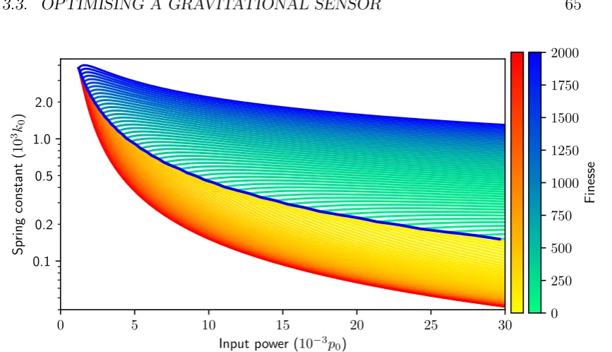
3.3.3 Sensitivity optimisation . . . 60
3.4 Conclusion . . . 66
4 Feedback cooling and retrospective filtering for nanomechanical sensors 69 4.1 Background . . . 70
4.2 A nanowire-based optomechanical force sensor . . . 72
4.2.1 Nanowires . . . 74
4.2.2 Detection . . . 75
4.2.3 Actuation . . . 75
4.2.4 Feedback control . . . 76
4.2.5 Force sensing . . . 79
4.3 Sensitivity enhancement . . . 84
4.3.1 Physical feedback cooling . . . 84
4.3.2 Virtual feedback cooling . . . 85
4.3.3 Kalman filtering . . . 89
4.3.4 Results . . . 94
4.3.5 Discussion . . . 97
4.4 Conclusion . . . 105
5 Automated optimisation with machine learning 107 5.1 Background . . . 108
5.1.1 Quantum control . . . 109
5.1.2 Optimisation via machine-learned models . . . 110
5.2 A scalable machine learning algorithm for automatic optimisation 111 5.2.1 Introduction to artificial neural networks . . . 112
5.2.2 Algorithm details . . . 123
5.3 Optimising a magneto-optical trap with machine learning . . . 130
CONTENTS xi
5.3.4 Discussion . . . 137 5.4 Conclusion . . . 155
Chapter 1
Introduction
Quantum optical systems are on the brink of a transition from experimental plat-forms to core components of cutting-edge commercial technologies. This transi-tion promises to unlock new possibilities in a range of fields, from informatransi-tion and communication technology to precision metrology. As quantum optical systems become integrated into applied technologies, high performance will become a key requirement. Proof-of-principal systems, while adequate in an experimental con-text, will not suffice; instead, components exhibiting optimal performance will be necessary. The transformation of a proof-of-principal system into a maximally-performant component suitable for a commercial device will entail system-wide optimisation.
Quantum optical systems are uniquely difficult to optimise. While quan-tum effects are precisely what enable the impressive capabilities of such systems, they also induce a range of challenges. For example, the Heisenberg uncertainty principle places intrinsic limits on the precision of measurements made on such systems. These limits manifest as quantum back action—the act of measurement itself perturbs the system, and this perturbation precludes precise knowledge of non-commuting observables. Improved manufacturing is not sufficient to over-come these challenges; instead, the devices must be fundamentally altered in order to sidestep the problematic quantum effects.
Not all quantum optical systems are amenable to the same styles of optimisa-tion. The additional complexities required to model quantum behaviour render even moderately complex systems intractable to detailed theoretical analysis. In such cases optimisation must proceed via approximate analysis based on those aspects of the system that are understood. For some systems even this approach
is infeasible, and one must instead revert to brute-force search. More generally, as system complexity increases, the required optimisation procedures become more general and less “physical”.
In this thesis we consider a selection of quantum systems sampled from this spectrum of complexity (and analytical intractability), and a corresponding col-lection of methods for optimising their performance.
1.1
Emerging quantum optical technologies
Optical systems have enjoyed a long history as a test bed for physical phenomena, from the famous Michelson-Morley experiment of 1887 through to the gravita-tional wave detectors of the present day. For quantum physics, in particular, the use of light is ubiquitous due to its general experimental convenience, its weak interaction with the environment, and the relative accessibility of quantum states and quantum effects.
The uses of quantum optical systems are not constrained to the realm of ex-perimental physics, however. The most well-known such system with widespread commercial applications is the laser, which has formed the basis for an astonishing array of modern technologies. To name just a few, the laser underpins everyday devices such as barcode scanners, laser printers and CD drives; medical apparatus including instruments for dentistry[1] and eye surgery[2]; industrial-scale machin-ery for processing a variety of materials from metals[3, 4] through to plastics[5] and carbon fibre[6]; and atomic force microscopes for nanoscale imaging[7, 8].
1.2. KEY TECHNICAL CHALLENGES 3
so on.
Already these technologies are receiving significant commercial attention, with companies today delivering quantum random number generators[17], gravime-ters[18], cold atom-based atomic clocks[19] and quantum key distribution sys-tems[20]. On the computation side the progress towards viable products is not so advanced, but if anything the interest and investment are even more intense. Large companies such as Google[21] and Lockheed Martin[22] are betting on the technology to enable breakthroughs in artificial intelligence and machine learn-ing, while there are a wide variety of start-ups looking to carve out more specific niches in the domain.1
1.2
Key technical challenges
Despite this promising start, there remain significant barriers to the widespread adoption of exotic quantum optical systems as components of the technologies of the future. One fundamental problem is that quantum optical systems are inher-ently fragile. While photons in free space retain quantum information remarkably well, any interaction with external systems quickly leads to a loss of information via decoherence, and for information technology applications it is often exactly this type of interaction that is required.
For secure communication via quantum key distribution, for example, inte-gration with existing fibre optic networks is desirable. However, losses in the fibre induce a loss of quantum information and lead to unacceptably low bit rates when used over large distances. Current telecom-grade low-loss optical fibre typ-ically exhibits attenuation on the order of 0.2 dB/km[27], which limits the range of a single hop in a useful quantum network to a few hundreds of kilometers[28]. Unlike with classical communication over optical fibre, the no-cloning theorem precludes the use of simple amplification to circumvent this issue. Instead, in-tegration of quantum repeaters into the network is expected to enable secure communication via multiple hops and thus bypass this limit[29–32], but while many of the individual components required to build a useful quantum repeater have been demonstrated, a complete system has not yet been realised. A
partic-1See, for example, Rigetti Computing[23] (full-stack quantum computing), h-bar[24] (general
consulting on quantum information technologies), QxBranch[25] (consulting on applications to
ular subsystem that we will discuss in more detail in Chapter 5 is the quantum memory. In brief, the memory used in a quantum repeater must exhibit storage times long enough to allow entanglement to be shared between distant nodes of the network, and the time required for this sharing depends on the memory ef-ficiency. For example, to achieve higher bit rates than direct fibre transmission over a distance of 500 km, a memory with 90% efficiency and storage time on the order of seconds is required[31]. A coherent optical memory with efficiency as high as 87% has been reported, but at this efficiency the storage time was on the order of microseconds[33]. Conversely, there are memories with storage times of seconds, but the efficiencies are below 1%[34, 35]. Indeed, the highest reported storage time for a memory with over 50% efficiency is 0.6 ms[36], indicating that there is still significant optimisation to be performed before a memory suitable for a useful quantum repeater becomes within reach.
Generally speaking the situation is not quite so intimidating for sensing ap-plications, and this is reflected by the relative maturity of commercial sensors based on quantum optics. Such systems typically have far fewer interacting com-ponents than large-scale quantum information processing devices, which signifi-cantly relaxes the degree of internal isolation required for reducing the effect of decoherence. Indeed, in many sensing applications it is not even necessary to have long coherence times in the first place. In addition, unlike in quantum key distribution systems designed to integrate with existing fibre optic networks, a sensor can usually be delivered as a single self-contained unit, which at least al-lows sources of noise within the system to be controlled. Despite these mitigating factors, however, quantum optical sensors still contain delicate components and configurations susceptible to the weakest environmental disturbances, so perfor-mance is highly sensitive to external noise sources. In addition to these noises there is yet another more fundamental source, namely the quantum back action, whereby the act of measurement itself can significantly disturb the system. Even this does not enforce a hard limit, however, and with creative system design and careful optimisation it is possible to evade the effect of back action and thus further improve performance, as we will discuss in Chapter 2.
ca-1.3. OPTIMISING QUANTUM OPTICAL SYSTEMS 5
pabilities will emerge, such as fault-tolerant computation[37, 38] or high-speed quantum communication across multiple network nodes[29, 30], while in sensing it is more a matter of gradual sensitivity enhancement. In both cases, however, it is clear that iterative optimisation of system performance is vital for further technological development and commercial adoption.
1.3
Optimising quantum optical systems
Optimisation of quantum optical systems entails some unique challenges. Speak-ing very generally, one common theme is that it can be difficult to optimise individual components in isolation. Typically the underlying problem is that sys-tems are so fragile that perturbations to one part of the system are sufficient to cause significant disturbances in others.
The Heisenberg uncertainty principle can be interpreted in this context: it is possible to decrease the noise in one observable, but doing so necessarily increases noise in any non-commuting observable.
A more concrete example, which will be the focus of Chapter 2, is found in long-baseline gravitational wave detectors. Injection of classical states of light into such devices leads to a strict sensitivity limit known as the “standard quantum limit”, which arises from the phase and amplitude noise in the light. Using quantum states of light, however, the limit can be beaten: injecting suitable squeezed light can improve the sensitivity at part of the detection band, at the expense of a reduction in sensitivity over the rest of the band[39]. In order to achieve improvement across the entire band (broadband improvement) one must not only squeeze the light, but ensure that the squeezed quadrature rotates with detection frequency. If perfect quadrature rotation is not possible, the squeeze factor must also be frequency-dependent in order to reduce the negative impact of anti-squeezing at parts of the spectrum where the quadrature angle is imperfect. That is, one must optimise the squeeze factor and angle simultaneously.
finesse is necessary. We will show that this tension can be resolved, but only with significant changes to the system design. The fundamental difficulty in this case is that the sensing and readout systems are tightly coupled, so must be optimised as a single unit.
To summarise, for quantum optical systems consisting of multiple physical or functional components one must often optimise the entire system as a whole. This process is fundamentally more difficult than when the components are loosely coupled and can be optimised in isolation.
An additional challenge is that quantum systems are inherently difficult to model, which means that many even moderately complex systems are largely in-tractable to useful theoretical analysis. When dealing with such a system one must essentially revert to a combination of simplified analysis, brute-force, intu-ition and serendipity. Framing this observation more generally, as the complexity of the system increases there is less chance that it will be possible to perform calculated, principled improvements based on theoretical analysis, and instead optimisation must be performed more as though the system is a black box with unknown dynamics. A corollary is that for more complex systems the relevant optimisation processes become more general and applicable to a wider variety of systems.
In this thesis we consider a collection of systems of varying complexity and generality, and a corresponding suite of optimisation techniques. Our discussions range from specific systems that are sufficiently well-understood that paths to op-timisation can be identified entirely by bespoke theoretical analysis, to broader classes of systems for which general but theoretically-grounded domain-specific techniques are beneficial, through to the most general case of systems that are so complex that they must be treated as unknown black boxes by the optimisa-tion procedure. Throughout this process we thus provide a selecoptimisa-tion of specific techniques suitable in each situation, and simultaneously demonstrate the more general principle that across the spectrum of system complexity and generality one must employ vastly different styles of optimisation.
1.4
Thesis outline
The remainder of this thesis is structured as follows.
1.4. THESIS OUTLINE 7
interferometer-based displacement detectors using non-classical light generated by optomechanical systems. Gravitational wave detectors, and interferometers in general, are limited by the quantum noise in the light used for measurement— a manifestation of the aforementioned quantum back action. At low powers and high frequencies the phase noise in the light induces photon shot noise at detection, while at high powers and low frequencies the amplitude noise ran-domly drives the test masses and can mask the signal. Injecting amplitude- or phase-squeezed light can thus reduce the noise floor at a particular part of the spectrum, but increases noise elsewhere due to the corresponding anti-squeezing. If the squeezed quadrature rotates with frequency then enhancement across the entire measurement band is possible. We demonstrate that the output field of optomechanical systems exhibits frequency-dependent squeezing, and investigate whether such light is suitable for use in gravitational wave detectors. Despite the complexity of the relevant systems and the technical difficulty in implement-ing them, this can be seen as an example of one of the cleanest approaches to optimising performance. Specifically, the system is sufficiently well-understood that a path to improving sensitivity is known, and all that remains is to iden-tify an auxiliary system with the appropriate behaviour. Moreover, the coupling between the original system and the auxiliary system is minimal—the auxiliary system affects the behaviour of the detector solely via the light field injected into the detector, so the two systems can largely be optimised independently.
In Chapter 3 we derive a scheme for synthesising arbitrary optical spring po-tentials in cavity optomechanical systems by utilising polychromatic light. We focus on how the scheme may be used to optimise the sensitivity of optical spring-based gravitational sensors. This approach is applicable to any cavity optome-chanical system, and has a wide variety of potential uses due to its generality. One particular fact we demonstrate is that by using this scheme one can essentially break the aforementioned coupling between the sensing and readout subsystems of optical spring sensors, by allowing the former to be manipulated arbitrarily without changing the cavity finesse. From a broad optimisation perspective the situation here is similar to the previous chapter, in the sense that the procedure is grounded on a detailed theoretical understanding of the system dynamics.
that the use of this system in a non-stationary feedback cooling strategy enables an enhancement in sensitivity to transient signals. Next we present two post-processing schemes, which can be viewed as simulations of the feedback cooling process, and demonstrate that they achieve a similar enhancement in sensitivity without the need for additional experimental complexity. These techniques can be viewed as a more general approach to optimisation than those derived in the previous chapters, in the sense that they could potentially be used in arbitrary oscillator-based sensors of transient forces, without an understanding of the full system-specific dynamics and subtleties.
In Chapter 5 we take a more general approach again, and present a machine learning algorithm capable of automatically performing multi-parameter optimi-sation of arbitrary physical systems. The algorithm takes control of a system or experiment, and through repeated interactions learns a model of its behaviour and uses this model to determine the optimal parameter set to achieve a certain objective. This approach largely abandons all physical intuition and knowledge, since the algorithm treats the physical system as a black box. This technique enables optimisation of systems that are too complex for any useful theoreti-cal analysis, with parameter spaces too large for brute-force search. As a proof of concept, we apply the algorithm to a magneto-optical trap with 63 tunable parameters.
Chapter 2
Interferometric sensitivity
enhancement via optomechanical
squeezing
In this chapter we demonstrate how cavity optomechanical systems may be used to generate squeezed light, and investigate the prospect of using such light to enhance the sensitivity of interferometer-based gravitational wave detectors.
In Section 2.1 we provide some background and history on interferometer-based detectors, with a focus on how their performance can be optimised with the injection of non-classical light. In Section 2.2 we derive expressions describing the squeezing characteristics of the output field of an idealised cavity optomechanics system. In Section 2.3 we use these expressions to numerically analyse some prop-erties of optomechanically-generated squeezed light, under realistic assumptions. In Section 2.4 we investigate the possibility of using such light to improve the performance of long-baseline gravitational wave detectors. Finally, in Section 2.5 we provide some concluding remarks.
The contents of this chapter are based on the following publication: G. Guccione, H. J. Slatyer, A. R. R. Carvalho, B. C. Buchler, and P. K. Lam, “Squeezing quadrature rotation in the acoustic band via optomechanics”, Journal of Physics B: Atomic, Molecular and Optical Physics 49, 065401 (2016)
All stages of the research described in this chapter were performed in close col-laboration between Giovanni Guccione and myself.
2.1
Background
Interferometry, the use of light interference for precision measurement, is the basis for many of the world’s most sensitive detectors. General improvements in design and quality have increased the performance of these detectors over the last century, but with the effect of classical noise sources now being drastically reduced we are beginning to enter an era in which the limits imposed by quantum mechanics become significant.
Heisenberg’s uncertainty principle represents the most fundamental limit to the sensitivity of a detector. In optics this principle dictates that the phase and amplitude of the light cannot simultaneously be known precisely. In an interfer-ometric system effecting a measurement of a field quadrature, this uncertainty manifests as the well-known shot (or photon counting) noise[39, 41, 42]. The effect of shot noise can be mitigated by increasing the power of the laser; the signal increases more rapidly with laser power than the noise, meaning a higher power yields an improved signal-to-noise ratio. However, a higher laser power yields a stronger radiation pressure force, and—particularly when free masses are involved—this back action can drive the optical components of the measurement apparatus and thus increase noise[43]. That is, even in the absence of experimen-tal limitations to the laser power there is a tradeoff to be made: a lower power reduces radiation pressure noise but increases shot noise, while a higher power decreases the effect of shot noise but increases radiation pressure noise. There is thus an optimal power at which to operate, where the combined contribution from radiation pressure noise and shot noise is minimised. This is known as the
standard quantum limit (SQL) for interferometers[44, 45].
To be noticeably affected by the SQL requires extreme optimisation of all other noise sources, but despite the technical difficulty this regime is now being explored. The most well-known detectors operating at this level are long-baseline gravitational wave detectors (see, for example, the recent review by Holst et al.[46]). The previous generation of detectors tended to operate at a low enough power to be limited by shot noise across the detection band[47], but the current generation are limited by the SQL at the optimal detection frequency[48].
2.1. BACKGROUND 11
contribute equally across the detection band. At high frequencies the radiation pressure noise is low due to being far from the mechanical resonances, so shot noise dominates, while at low frequencies the situation is reversed. Therefore, if one can reduce the effect of either shot noise or radiation pressure noise then the noise floor at the appropriate part of the spectrum will be reduced. It is here that squeezing can be advantageous. By using phase-squeezed light, for example, the shot noise is reduced and the sensitivity at high frequencies improves. Indeed, this technique has already been used to beat the shot noise limit in interferometers[53– 56]. However, such light also exhibits anti-squeezing in the amplitude quadrature, which leads to higher radiation pressure noise and thus increased noise at low frequencies, so once again there is a tradeoff. Similarly, injecting amplitude-squeezed light (or indeed light amplitude-squeezed at any fixed angle) sacrifices sensitivity at some frequencies in order to improve it at others.
pri-mary technical difficulty with traditional filter cavities, namely an extremely low linewidth.
In all of these approaches the idea is first to generate fixed-angle squeezed light using established techniques (see, for example, the review by Anderson et al.[69]) and then filter this light to achieve quadrature rotation. In this chapter we consider an alternative approach, which is to inject squeezed light generated by an optomechanical system directly into the interferometer[70–72]. As we will show, such light naturally exhibits frequency-dependent quadrature rotation due to the dispersive optomechanical interaction, and, moreover, this effect occurs over a frequency band determined by the mechanical frequency, which can quite naturally fall in the acoustic band.
We will demonstrate that with a suitable choice of parameters, within reach of current state-of-the-art systems[73–75], such a scheme can provide an alternative to filter cavities and fixed-angle squeezing for use in long-baseline gravitational wave detectors. There is a fundamental limitation, however, which is that the frequency-dependent quadrature rotation occurs in the opposite direction to that required for optimal improvement. Combined with the high anti-squeezing occur-ring in the orthogonal quadrature, this precludes sensitivity enhancement across the full detection band. Unlike in the case of fixed-angle squeezed light, it is possible to attain a modest improvement at both high and low frequencies simul-taneously, but this would only be potentially useful in specific (unusual) modes of operation. Thus our proposal is not suitable as a general-purpose method for optimising gravitational wave detectors.
2.2
Calculation of the output spectrum for
op-tomechanical squeezing
2.2. OUTPUT SPECTRUM CALCULATION 13 ˆ ain ˆ aout ˆ a m ωm
L0 xˆ
Figure 2.1: Basic optomechanical system. The left-hand cavity mirror is fixed, while the right-hand mirror is moveable and lies in a harmonic potential. The labels are defined in the text.
2.2.1
Output field
We consider a linear optical cavity of equilibrium lengthL0 with one fixed mirror and one moveable mirror with natural mechanical frequency ωm and mass m, as shown in Fig. 2.1.
For simplicity we consider the limit in which the natural mechanical frequency is significantly slower than the cavity free spectral range (the spacing between cavity modes, given by ωFSR := πcL0). This allows us to ignore the scattering of photons into different cavity modes stimulated by the optomechanical interaction, and thus confine the analysis to a single cavity mode[76, 77].
Let the input laser frequency be ωopt and the equilibrium cavity resonance frequency beω0, and define the equilibrium cavity detuning ∆0 :=ωopt−ω0. Let ˆ
a and ˆa†be the respective annihilation and creation operators for the field inside the cavity. Let ˆxbe the displacement of the moveable mirror from its equilibrium position, let ˆp be the mirror momentum, and let ω(ˆx) be the cavity resonance frequency for a given displacement.
Basic equations of motion
It will be convenient to work in a frame rotating at the optical frequency ωopt, so we have the Hamiltonian
ˆ
H =~(ω(ˆx)−ωopt)
ˆ
a†ˆa+1 2
+ pˆ 2
2m +
1 2mω
2 mxˆ
2
. (2.1)
We may approximate
ω(ˆx)≈ω0−
ω0
L0 ˆ
where we have defined the basic optomechanical coupling strength G0 according to
G0 :=−
∂ω(ˆx)
∂xˆ
0 = ω0
L0
. (2.3)
This term converts a mirror displacement into a shift in resonance frequency, and thus describes the strength of the optomechanical interaction. The Hamiltonian simplifies to
ˆ
H≈~(−∆0−G0xˆ)
ˆ
a†ˆa+ 1 2
+ pˆ 2
2m +
1 2mω
2 mxˆ
2
≈ −~∆0ˆa†aˆ−~G0xˆˆa†ˆa+ ˆ
p2
2m +
1 2mω
2
mxˆ2, (2.4)
where in the second line we have omitted the contribution from the vacuum. From this and the commutation relations
[ˆa,ˆa†] = 1, [ˆx,pˆ] =i~, [ˆa,xˆ] = [ˆa,pˆ] = 0 (2.5)
we can calculate the equations of motion for the Heisenberg-picture operators in the absence of any noise or input:
˙ˆ
x= i
~
−i~pˆ
m
= pˆ
m (2.6)
˙ˆ
p= i
~ −
i~2G0ˆa†aˆ+ 2i~mωm2xˆ=~G0ˆa†aˆ−mω2mxˆ (2.7) ˙ˆ
a= i
~(~∆0ˆ
a+~G0xˆˆa) =i(∆0+G0xˆ)ˆa. (2.8)
Accounting for noise and inputs
To complete the picture we must include terms accounting for the mechanical and optical losses, and the driving input field.
Let the cavity half-linewidth be κ. We consider the adiabatic limit, where
2.2. OUTPUT SPECTRUM CALCULATION 15
The full equations of motion, which are known as the quantum Langevin equations (see Gardiner and Zoller[78] for further discussion), are thus
˙ˆ
x= pˆ
m (2.9)
˙ˆ
p=~G0ˆa†ˆa−mωm2xˆ−γpˆ+ ˆF (2.10) ˙ˆ
a=i(∆0+G0xˆ)ˆa−κˆa+
√
2κaˆin. (2.11)
Linearising the system
We will simplify the analysis by considering only small perturbations of the op-erators from their steady state values. We first calculate the steady state (x, p, a) based on the mean input field ain and thermal drivingF = 0:
˙ˆ
x= 0 =⇒ p= 0 (2.12)
˙ˆ
p= 0 =⇒ ~G0a∗a−mω2mx= 0
=⇒ x= ~G0|a| 2
mω2 m
(2.13) ˙ˆ
a= 0 =⇒ i(∆0+G0x)a−κa+
√
2κain = 0
=⇒ a =−
√
2κain
i(∆0 +G0x)−κ
(2.14)
Next we introduce the perturbations from the mean steady states:
δxˆ:= ˆx−x (2.15)
δˆa:= ˆa−a (2.16)
Plugging into Eqs. (2.9) to (2.11) (and recalling that ˆain=ain+δˆain) we obtain
˙
δxˆ= ˙ˆx= pˆ
m (2.17)
˙ˆ
p=~G0 a∗+δˆa†
(a+δˆa)−mωm2 (x+δxˆ)−γpˆ+ ˆF (2.18) ˙
δˆa= ˙ˆa=i(∆0+G0(x+δxˆ)) (a+δaˆ)−κ(a+δˆa) +
√
which can be expanded and then simplified via Eqs. (2.12) to (2.14):
˙ˆ
p=~G0a∗a−mω2mx+~G0 a∗δˆa+aδˆa†+δaˆ†δaˆ
−mωm2δxˆ−γpˆ+ ˆF
=~G0 a∗δˆa+aδaˆ†+δˆa†δˆa
−mω2mδxˆ−γpˆ+ ˆF (2.20) ˙
δaˆ=i(∆0+G0x)a−κa+
√
2κain
+i(∆0+G0x)δˆa+iG0aδxˆ+iG0δxδˆ ˆa−κδaˆ+
√
2κδaˆin =i(∆0+G0x)δˆa+iG0aδxˆ+iG0δxδˆ ˆa−κδˆa+
√
2κδaˆin = (i∆−κ)δˆa+iG0aδxˆ+iG0δxδˆ ˆa+
√
2κδˆain, (2.21)
where in the last line we have defined ∆ := ∆0+G0x to be the detuning at the steady state position.
We observe that applying a phase shift to the input fieldsain and δˆain causes a corresponding phase shift in a, and these shifts may then be absorbed intoδˆa. That is, by varying the phase of the input field we may arbitrarily shift the phase of the intra-cavity field fluctuations δˆa. Thus for our calculations we can assume that the input phase is chosen to makea positive and real, while knowing that in practice we may shift the reference phase of δˆa arbitrarily by shifting the phase of the input field.
We now define the adjusted optomechanical coupling strength G := G0a, which converts a displacement into the combined frequency shift for the whole (mean) intra-cavity field. Assuming a 1 (that is, the number of photons circulating in the cavity is high) we may omit the second-order perturbation terms and thus obtain the linearised equations of motion:
˙
δxˆ= pˆ
m (2.22)
˙ˆ
p=~G δˆa+δˆa†
−mω2mδxˆ−γpˆ+ ˆF (2.23) ˙
δaˆ= (i∆−κ)δˆa+iGδxˆ+√2κδˆain. (2.24)
Solving the system
To solve this system of equations we first apply the Fourier transform
F(f)(ω) :=
Z ∞
−∞
2.2. OUTPUT SPECTRUM CALCULATION 17
For clarity of notation we use the same symbol for an operator and its Fourier transform, but there will be no ambiguity since from this point on we will only ever be working in the frequency domain unless explicitly stated otherwise. Similarly, we will usually drop the argument to operators when it is simply ω. For an operator f we denote f† ≡ f†(ω) ≡ F(f†)(ω); that is, the Fourier transform of the conjugate as opposed to the conjugate of the Fourier transform. The system becomes
iωδxˆ= pˆ
m (2.26)
iωpˆ=~G δˆa+δaˆ†−mωm2δxˆ−γpˆ+ ˆF (2.27)
iωδˆa= (i∆−κ)δˆa+iGδxˆ+√2κδˆain. (2.28)
To solve for the cavity field δaˆ we start by eliminating ˆp from the first two equations to obtain
χ−m1(ω)δxˆ=~G δˆa+δˆa†+ ˆF , (2.29)
where we have defined the standard mechanical susceptibility
χm(ω) :=
m ωm2 −ω2+iγω−1, (2.30)
which describes the response of the oscillator to a unit impulsive force in the absence of any optomechanical interaction.
The equation for δaˆ can be written in the form
δˆa=χopt(ω)iGδxˆ+√2κδˆain
, (2.31)
where we have defined the optical susceptibility
χopt(ω) := (iω−i∆ +κ)−1, (2.32)
which describes the response of the optical cavity to an injected photon (if we fix the moveable mirror in its steady state position).
δˆa†:
δˆa†(ω) = δˆa(−ω)†
=χopt(−ω)∗−iGδxˆ(−ω)†+√2κδaˆin(−ω)†
=χ∗opt(ω)−iGδxˆ(ω) +√2κδˆa†in(ω), (2.33)
where for the last line we have used Hermiticity of δxˆand defined
χ∗opt(ω) := (iω+i∆ +κ)−1 =χopt(−ω)∗. (2.34)
Now we may substitute the expressions forδaˆandδˆa†into Eq. (2.29) to obtain
χm(ω)−1δxˆ=
~G h
χopt(ω)iGδxˆ+√2κδaˆin
+χ∗opt(ω)−iGδxˆ+√2κδaˆ†ini+ ˆF ,
(2.35)
which can be rearranged to
χm(ω)−1
−i~G2 χopt(ω)−χ∗opt(ω)
δxˆ=
√
2κ~Gχopt(ω)δaˆin+χ∗opt(ω)δˆa
†
in
+ ˆF . (2.36)
From this we can define the effective mechanical susceptibility
χeff(ω) :=
χm(ω)−1−i
~G2 χopt(ω)−χ∗opt(ω)
−1
, (2.37)
which describes the full response of the oscillator, in the presence of the optome-chanical interaction, to an impulsive force. We observe that the optomeoptome-chanical interaction causes a frequency-dependent shift in the effective mechanical fre-quency and linewidth[79, 80]:
ωeff(ω)2 :=ω2
m+
~G2
m =
χopt(ω)−χ∗opt(ω)
(2.38)
γeff(ω) := γ−~G
2
mω<
χopt(ω)−χ∗opt(ω)
. (2.39)
Note that for ω κ these quantities are essentially constant with respect to ω, so usually we omit the ω argument and treat them as constants (with respect to
2.2. OUTPUT SPECTRUM CALCULATION 19
Continuing from Eq. (2.36) we obtain
χeff(ω)−1δxˆ=√2κ~Gχopt(ω)δˆain+χ∗opt(ω)δaˆ
†
in
+ ˆF . (2.40)
Substituting into Eq. (2.31) we can express the cavity field in terms of only the inputs:
δˆa=χopt(ω)
iGχeff(ω)h√2κ~G
χopt(ω)δˆain+χ∗opt(ω)δˆa
†
in
+ ˆF
i
+√2κδˆain
.
(2.41)
By invoking the input-output relation[81] δaˆout =
√
2κδˆa−δˆain and rearranging we obtain the output field:
δaˆout =
√
2κiGχopt(ω)χeff(ω)h√2κ~G
χopt(ω)δˆain+χ∗opt(ω)δˆa
†
in
+ ˆF
i
+ (2κχopt(ω)−1)δaˆin =
2κi~G2χeff(ω)χopt(ω)2+χopt(ω)/χ opt(ω)∗
δˆain + 2κi~G2χeff(ω)χopt(ω)χ∗opt(ω)δˆa†in
+√2κiGχeff(ω)χopt(ω) ˆF ,
(2.42)
where we have observed that 2κχopt(ω)−1 = χopt(ω)/χopt(ω)∗. Similarly, the
conjugate is given by
δˆa†out =
2κi~G2χeff(ω)χ∗opt(ω)2+χ∗
opt(ω)/χ
∗
opt(ω)
∗
δˆa†in
+ 2κi~G2χeff(ω)χopt(ω)χ∗opt(ω)δˆain +√2κiGχeff(ω)χ∗opt(ω) ˆF .
(2.43)
Observations
Before calculating the output spectrum, which will be our main tool for analysing the properties of this output field, we can make some initial observations from simply inspecting Eq. (2.42). This will provide intuition that can guide the choice of parameters in the subsequent sections.
First, in the case that G ≈ 0 (that is, the mechanical motion has a negligi-ble effect on the optical properties of the system), only the χopt(ω)/χopt(ω)∗δˆa
2 arg(χopt(ω)) = 2 arctan((∆ −ω)/κ) to the input field. In particular, if this input field is squeezed then the cavity will perform a frequency-dependent rota-tion of the squeezed quadrature, which is the basis of approaches to generating quadrature rotation based on filter cavities (see Section 2.1). We can also see one reason why these schemes are challenging: to achieve a significant phase shift over a 100 Hz band we must have a linewidth κ/2π on the order of 50 Hz (or even lower), which corresponds to a cavity storage time of several milliseconds. Such cavities have only just started to become within reach of experimental realisa-tion[64].
WhenG6≈0 the dynamics become significantly more interesting. Specifically, one may observe that the output field depends on both the noise in the input field and its conjugate, so a priori we may be able to choose parameters to make these terms interfere destructively. By doing this we would reduce the noise in one component of the output field and thus generate squeezed light. Moreover, since the coefficients are frequency-dependent, the maximally-squeezed quadrature would rotate with frequency. Finally, since the coupling terms are proportional to the mechanical susceptibility, this suggests that any generated squeezing will be near the mechanical frequency.
In fact, we can extract further insight by inspecting the first two terms of Eq. (2.42), which we denote δˆasqzout, in more detail. One may notice that the first two terms resemble the action of the squeeze operator on the input field. The squeeze operator[82, 83],
ˆ
S(r, φ) := exphr 2
e−2iφˆa2 −e2iφaˆ†2
i
, (2.44)
acts on the vacuum (or any coherent state) to reduce the noise in theφquadrature by a factor of e−2r and increase the noise in the orthogonal quadrature by e2r. We refer to r as thesqueeze factor and φ as thesqueeze angle. The action of the squeeze operator on the field operator ˆa is given by
ˆ
S(r, φ)†ˆaSˆ(r, φ) = coshraˆ
−e2iφsinhraˆ†. (2.45)
Thus we see that, if an appropriate choice of squeeze factor r and angleφ can be made,δaˆsqzoutindeed describes a (scaled) squeeze of the input vacuum fluctuations.1
1If the reader is unfamiliar with the squeeze operator, for the sake of intuition one can
2.2. OUTPUT SPECTRUM CALCULATION 21
Specifically, abbreviating the coefficients of the first two terms in Eq. (2.42) as
α(ω) := 2κi~G2χeff(ω)χopt(ω)2+χopt(ω)/χopt(ω)∗ (2.46)
β(ω) := 2κi~G2χeff(ω)χopt(ω)χ∗opt(ω), (2.47)
we may write
δˆasqzout =α(ω)δˆain+β(ω)δˆa
†
in
=c(ω)coshr(ω)δˆain−e2iφ(ω)sinhr(ω)δˆa
†
in
, (2.48)
where we take
r(ω) := coth−1
α(ω)
β(ω)
, φ(ω) := π 2 +
arg(β(ω))−arg(α(ω))
2 ,
c(ω) := α(ω) coshr(ω).
(2.49)
For some choices of parameters this identification is not possible. Indeed, it is clear from the definitions that a sufficient condition is |α| > |β|, and if we recall that the hyperbolic functions satisfy cosh2x
− sinh2x = 1 we see that
|α|2 − |β|2 = |c|2 and thus this condition is also necessary. Some computation yields
|α(ω)|2− |β(ω)|2 = 1 + 4κG2~|χopt(ω)|2|χeff(ω)|2mγω, (2.50) so it is not hard to convince oneself that the condition could be violated, for example by considering frequencies within a linewidth of the effective mechanical frequency in systems with low mechanical damping rates. We will discuss this further when considering a specific system in Section 2.3.
Assuming we can indeed achieve the representation in Eq. (2.48), and contin-uing to ignore the contribution of the thermal spectrum to the output field, we can gain intuition about the magnitude and quadrature of the squeezing effect by considering the values of r and φ. Specifically, let us consider the case where
κ ω, which is the most interesting one for our purposes, since otherwise we
and the form of δˆasqzout reduces to d(ω)(δˆain+δˆa†in) +δˆain (for some d(ω)). This represents a
could simply use the cavity as a filter (as mentioned above). In this limit we can consider χopt to be independent of ω, and we also have χopt∗ (ω) ≈ χopt(ω)
∗. We
can therefore approximate
β(ω)≈2κi~G2χeff(ω)|χopt|2 (2.51)
α(ω)≈2κi~G2χeff(ω)χ2opt+χopt/χ∗opt = χopt
χ∗opt 2κi~G
2χeff(ω)|χ opt|
2 + 1
≈ χopt
χ∗opt (β(ω) + 1). (2.52)
If we further assume γ ωm, which is to say the mechanical resonator is of high quality, then we see that the effective susceptibility χeff is almost purely real (except when very close to the effective mechanical frequency), meaning β is essentially purely imaginary. A depiction of howαandβ lie in the complex plane is shown in Fig. 2.2. It will be illustrative to consider how this picture varies as the frequency ω is increased from 0 to ω ωeff. Initially the susceptibility χeff increases and thus the magnitude ofβ increases, with very little change in phase. As the effective mechanical frequency is approached the magnitude becomes very large (proportional to 1/γ), until near the effective mechanical frequencyβrotates through the positive real half-plane to lie on the negative imaginary axis. After this point the dynamics are reversed, and as ω increases further the magnitude of β decreases back towards 0. With this picture we can gain some intuition into how the squeezing of the system varies with parameters.2
Looking first at the definition of the squeeze factor r given in Eq. (2.49), we see that to maximise the squeeze factor we must bring the ratio |α/β|as close to unity as possible, which, given our approximations, is simply a case of maximising
|β|. This suggests that the maximum attainable squeezing level, which should be achieved near the effective mechanical frequency, will increase by decreasing any of the mechanical damping, optical linewidth κ or detuning |∆|.
Now let us consider the angle of squeezing, where in particular we will be concerned with the change in squeezed angle asωvaries. First note that following
2We also refer the reader to an elegant alternative approach to visualising the behaviour of
2.2. OUTPUT SPECTRUM CALCULATION 23
1
β(0) α(0)
β(< ωeff) α(< ωeff)
β(∼ωeff)
β(> ωeff) α(> ωeff)
ψ(0)−c.t.
<(z)
[image:35.595.138.501.188.495.2]=(z)
Figure 2.2: Illustration of coefficients α and β in the limit of large optical linewidth and small mechanical linewidth. For simplicity we have considered the case where χopt is approximately real (that is, ∆ = 0); in the general case
α would be rotated by 2 arg(χopt). We have α(ω) = β(ω) + 1 for all ω. As ω
the squeeze S(r(ω), φ(ω)) there is a scale by c(ω), which may be complex and thus effect a rotation of the squeezed field, so the squeezed angle ψ(ω) of the output field is given by
ψ(ω) = arg(c(ω)) +φ(ω) = arg(α(ω)) +φ(ω) = π
2 +
arg(β(ω)) + arg(α(ω)) 2
= π
2 + arg(χopt) +
arg(β(ω)) + arg(β(ω) + 1)
2 . (2.53)
The first two terms are independent ofω, so to achieve a large amount of squeezing angle rotation we must cause the average phase of β and β+ 1 to vary as much as possible. Thinking of this in terms of the picture described above we see that, ignoring the constant terms, the initial squeezing angle is determined by the initial magnitude of β: for a small magnitude we will have an angle close toπ/4, while for a larger magnitude this will increase towards π/2. As ω increases the angle tends to π/2, until the effective mechanical frequency is reached at which point the picture is reflected and the angle jumps to −π/2. Then as we increase
ω further the angle will tend back towards −π/4. Thus the factor determining the total amount of quadrature rotation across the spectrum is the magnitude of
β at the start and end of the spectrum. We may decrease this magnitude, and thus increase the total amount of quadrature rotation towards π/2, by increasing the mechanical frequency, optical linewidthκ or detuning |∆|. Note the contrast to the squeezing factor, which decreases asκ and |∆| increase.
To conclude our initial observations, we note an interesting property of the system’s action on commutation relations. Since the squeezing operator is unitary, and thus preserves commutation relations, it may appear from Eq. (2.48) that if
2.2. OUTPUT SPECTRUM CALCULATION 25
level.
2.2.2
Output spectrum
To explore the behaviour of the output field (given by Eq. (2.42)) in more detail we may calculate the power spectra for its individual quadratures.
Noise correlation functions
The first step is to specify the details of the driving noise terms, namely the input vacuum fluctuationsδˆainand the force from the thermal bath ˆF. We assume that the optical drive is at room temperature, so ~ωopt kBT and thus the mean thermal photon occupation nth
o is negligible. Moreover, the field fluctuations are essentially Markovian for a small bandwidth about optical frequencies[81, 85], meaning the correlation functions are
D
δˆa†in(ω)δˆain(ω0)E= 2πδ(ω+ω0)ntho
≈0 (2.54)
D
δˆain(ω)δˆa†in(ω0)E= 2πδ(ω+ω0)(ntho + 1)
≈2πδ(ω+ω0) (2.55)
hδˆain(ω)δaˆin(ω0)i=Dδaˆ†in(ω)δˆa†in(ω0)E= 0, (2.56)
where h·i denotes the expected value andδ is the Dirac delta function.
For the mechanical noise the situation is less straightforward, since in the quantum case Brownian forces are non-Markovian[78, 85, 86]. Specifically, we have the correlation function
D
ˆ
F(ω) ˆF(ω0)E= 2πδ(ω+ω0)Sth(ω), (2.57)
where the thermal noise spectrumSth is defined, following the analysis in [85], to be
Sth(ω) :=mγ~ω
coth
~ω
2kBT
−1
. (2.58)
spectrum can therefore be approximated as
Sth(ω)≈mγ~ω
1 + 2kBT
~ω
≈2mγkBT. (2.59)
Output spectrum for an arbitrary quadrature
We define the quadrature with angle θ as
ˆ
Xθ =e−iθδˆaout+eiθδaˆ
†
out. (2.60)
We define the symmetrised spectral density (see Clerk et al.[87] for a comprehen-sive discussion of noise spectra) of such a quadrature ˆXθ, normalised to the shot
noise, to be
Sθ(ω) := Z ∞ −∞ dω0 2π Dn ˆ
Xθ(ω),Xˆθ(ω0) oE
, (2.61)
where {·,·} denotes symmetrisation: {f, g}:= (f g+gf)/2.
Using Eqs. (2.42) and (2.43) for the output fieldδˆaout and its conjugateδˆa
†
out, together with the noise correlation functions Eqs. (2.54) to (2.57), we can deter-mine Sθ for an arbitrary θ. Some computation, which is rather tedious and not
particularly instructive (and hence omitted), yields
Sθ(ω) = 2κG2|χeff(ω)|
2
Sth(ω) +κ~2G2|χopt(ω)|2+χ∗opt(ω)
2
×
χopt(ω)−e2iθχ∗opt(ω)
2
+ 4κ~G2<[χeff(ω)]=
e2iθχopt(ω)∗χ∗opt(ω)
+ 2κ~G2=[χeff(ω)]
χ∗opt(ω)
2
− |χopt(ω)|2 + 1.
(2.62)
Squeezing angle and minimised spectrum
Fortunately the dependence of Eq. (2.62) on θ is quite simple, so some further calculations yield the quadrature angle θmin(ω) minimising the spectrum (and thus maximising squeezing):
θmin(ω) = π 2 +
1
2arctan2
(κ2+ω2−∆2)ξ(ω)−4κ∆ζ(ω)
−2(κ2+ω2−∆2)ζ(ω)−2κ∆ξ(ω)
2.3. PROPERTIES OF OPTOMECHANICAL SQUEEZING 27
where arctan2 yx
:= arg(x+iy) and we have abbreviated the coefficients of the two θ-dependent terms in Eq. (2.62) according to
ζ(ω) := 2κG2|χeff(ω)|2Sth(ω) +κ~2G2
|χopt(ω)|2 +χ∗opt(ω)
2
(2.64)
ξ(ω) := 4κ~G2<[χeff(ω)]. (2.65)
We can also define
Smin(ω) := Sθmin(ω)(ω) (2.66)
to be the value of the spectrum at the optimal angle, for each frequency. We can interpret θmin(ω) and Smin(ω) as the squeeze angle and factor for frequency ω.
2.3
Properties of optomechanical squeezing
With the noise spectrum Eq. (2.62) in hand we can investigate some properties of optomechanical squeezing. In particular, of course, we will focus on how the level and angle of squeezing vary with frequency in parameter regimes suitable for gravitational wave interferometry.
The parameters we use for the analysis and throughout the remainder of the chapter are shown in Table 2.1. Note that we have introduced several pa-rameters commonly used for characterising optomechanical systems, and from which all parameters in the above analysis can be deduced. Specifically: the quality factor of the mechanical resonator, Qm := ωm/γ; the total input laser
power, Pin := ~ωopt|ain| 2
; the laser wavelength, λ := 2πc/ωopt; the cavity fi-nesse, F = ωFSR/2κ; and the single-photon optomechanical coupling strength,
g0 := G0
p
~/2mωm. We have chosen to consider a cavity with medium finesse
Parameter Symbol Value
Mechanical frequency ωm 2π×150 Hz
Mechanical quality factor Qm 5×10⁶
Mirror mass m 0.5 kg
Temperature T 3 mK
Input power Pin 20 W
Wavelength λ 1064 nm
Free spectral range ωFSR 2π×1 GHz
Cavity damping κ 2π×0.5 MHz
Finesse F 1000
Single-photon OM coupling g0 2π×0.63 mHz
Test masses (LIGO) mgw 40 kg
Cavity length (LIGO) Lgw 4 km
Cavity damping (LIGO) κgw 2π×100 Hz
Table 2.1: Parameters used for the analyses of optomechanical squeezing and interferometric sensitivity enhancement.
followed by a rotation, followed by the addition of thermal effects.
With these parameters fixed we may calculate the spectrum in a few different scenarios. Specifically, we are looking to achieve squeezing in the acoustic band below around 300 Hz and ideally a quadrature rotation through an angle of π/2 across this band, since this is the behaviour required for optimising long-baseline gravitational wave detectors.
2.3. PROPERTIES OF OPTOMECHANICAL SQUEEZING 29
50 100 150 200 250 300 ω/2π(Hz)
−2.0
−1.5
−1.0
−0.5 0.0 0.5 1.0 1.5 2.0
∆
/κ
−10 −5 0 5 10 15 20 25 30
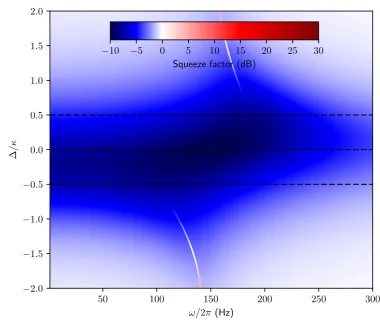
[image:41.595.124.505.216.536.2]Squeeze factor (dB)
50 100 150 200 250 300 ω/2π(Hz)
−2.0
−1.5
−1.0
−0.5 0.0 0.5 1.0 1.5 2.0
∆
/κ
0 π/4 π/2 3π/4 π
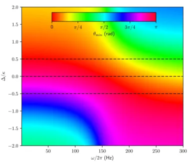
[image:42.595.88.475.110.434.2]θmin(rad)
Figure 2.4: Squeezing angle θmin(ω) for various detunings. Three specific detun-ings ∆ = −0.5κ,0,0.5κ are marked.
see that the squeezing factor diminishes as the frequency becomes too far from the mechanical frequency, again because the effect of the optomechanical interaction is attenuated by the low mechanical susceptibility.
We can similarly view the squeezing angle as a function of frequency and detuning, as shown in Fig. 2.4. As with the squeezing factor, the rotation of the squeezed angle generally tends to occur in the vicinity of the mechanical frequency. Unlike with the squeezing factor, however, a stronger rotation effect (that is, rotation through a larger angle) occurs with larger detunings. That is, there is a tradeoff to be made between the squeeze factor and the amount of quadrature rotation: detuning further from the cavity resonance increases the amount of rotation but decreases the squeeze factor across the band.
2.3. PROPERTIES OF OPTOMECHANICAL SQUEEZING 31 −10.0 −7.5 −5.0 −2.5 0.0 Squeeze facto r (dB)
∆ =−0.5κ
−10.0 −7.5 −5.0 −2.5 0.0 Squeeze facto r (dB)
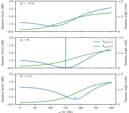
∆ = 0κ S
min(ω)
θmin(ω)
0 50 100 150 200 250 300 ω/2π(Hz) −10.0 −7.5 −5.0 −2.5 0.0 Squeeze facto r (dB)
∆ = 0.5κ
[image:43.595.117.533.203.567.2]0 π/4 π/2 Squeeze angle (rad) 0 π/4 π/2 Squeeze angle (rad) 0 π/4 π/2 Squeeze angle (rad)
plots we again see the tradeoff between squeeze factor and the total amount of quadrature rotation. Similarly, we can see more clearly that the interesting dynamics—high squeezing and quadrature rotation—both occur in the vicinity of the mechanical frequency, meaning if one desires good squeezing then one must also deal with the steady rate of quadrature rotation (and conversely). This observation will be important in the next section when we consider the use of optomechanically-squeezed light for gravitational wave detectors.
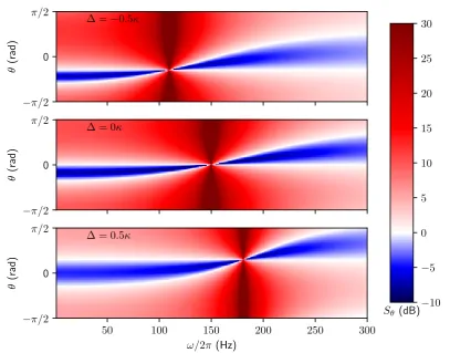
As discussed in Section 2.2.1 the light ejected from the cavity is not purely squeezed—there is additional noise due to the thermal effects (and, at least in a very narrow band about the effective mechanical frequency, due to the op-tomechanical interaction too). Therefore it is important to understand the full spectrum of noise, not only that in the squeezed quadrature. In Fig. 2.6 we plot the spectra of all quadratures as a function of angle for specific detunings. We see that, especially near the effective mechanical frequency (where the noise is resonantly amplified), significant anti-squeezing occurs. Combined with the observation above, that in order to have squeezing one must be near the me-chanical frequency and thus also have quadrature rotation, this suggests a dif-ficulty with the use of optomechanically-generated squeezed light in practice: unless the quadrature rotation is perfectly matched to the appropriate system, significant contamination could occur from the anti-squeezing and thus degrade performance.
2.4
Enhancement of LIGO sensitivity via
op-tomechanical squeezing
In this section we investigate how we expect the sensitivity of the Laser Interfer-ometer Gravitational-Wave Observatory (LIGO) to be affected by the injection of optomechanically-generated squeezed light.
2.4. LIGO SENSITIVITY ENHANCEMENT 33
−π/2
0
π/2
θ
(rad)
∆ =−0.5κ
−π/2
0
π/2
θ
(rad)
∆ = 0κ
50 100 150 200 250 300 ω/2π(Hz)
−π/2
0
π/2
θ
(rad)
∆ = 0.5κ
Sθ (dB)−
10
−5 0 5 10 15 20 25 30
Figure 2.6: Quadrature spectrum Sθ(ω) for all angles and specific detunings.
Notice that there is significant anti-squeezing in the vicinity of the effective me-chanical frequency.
Laser: Pgw
LIGO
Lgw
[image:45.595.116.524.122.441.2]Injection to dark port OM squeezing
2.4.1
The standard quantum limit
As discussed in Section 2.1, the sensitivity of the current LIGO detectors is limited by quantum noise across much of the detection band. This limit arises from shot noise—which introduces fluctuations in the detected output field—at high frequencies, and from radiation pressure noise—which randomly drives the test masses—at low frequencies.
For each given frequency there is an optimal power at which the contributions from these two noise sources agree and their sum is minimised: further increasing the power increases the contribution of radiation pressure noise and increases the total noise, while decreasing the power increases the shot noise and also leads to an increase in total noise. This point is the standard quantum limit (SQL). To see more quantitatively how the limit arises, we note that the noise spectrum for the conventional LIGO interferometer when vacuum is injected into the dark port, assuming all non-quantum noise to be negligible, is[45]
SLIGO(ω) = 8~
L2
gwmgwω2 × 1 2
1
K(ω) +K(ω)
, (2.67)
where K is a coupling constant describing how input fluctuations are coupled to output fluctuations via the radiation pressure force and the test masses, given by
K(ω) :=Pgw×
4ωopt
L2
gwmgwκ4gw
× 2κ
4 gw
ω2(κ2
gw+ω2)
. (2.68)
Looking at the expression in parentheses of Eq. (2.67), the K term describes the contribution of radiation pressure noise (as the optomechanical coupling increases, the fluctuations in the light are more strongly imprinted onto the test mass mo-tion), while the 1/Kterm describes the shot noise (the signal increases with higher optomechanical coupling, and thus the effect of shot noise decreases[88]). If we fix all parameters except the input power Pgw then it is clear that the spectrum is minimised, and thus the SQL is attained, when we have K(ω) = 1. That is (defining PSQL(ω) to be the appropriate operating power), we have
PSQL(ω) := L 2
gwmgwκ4gw 4ωopt ×
ω2 κ2 gw+ω2
2κ4 gw
2.4. LIGO SENSITIVITY ENHANCEMENT 35
20 50 100 200 500 1000 ω/2π(Hz)
−10
−5 0 5 10 15 20
Sensitivit
y
ratio
(dB)
SQL
[image:47.595.138.500.117.321.2]Conventional LIGO
Figure 2.8: Sensitivity of conventional LIGO interferometer when configured to reach the SQL at the optimal detection frequency, compared to the full spectrum of the SQL. The sensitivity ratio is defined as the square root of the appropriate spectral density normalised to the square root of the spectral density at the optimal detection frequency (SSQL(κgw)).
and the spectrum of the SQL is then given by
SSQL(ω) = SLIGO(ω)
Pgw=PSQL =
8~
L2
gwmgwω2
. (2.70)
We will typically be interested in optimising the performance for signals in the vicinity of the linewidthκgw, which we refer to as theoptimal detection frequency
(κgw= 2π×100 Hz for LIGO), so we henceforth assume Pgw to be the operating power required to reach the SQL at this point:
Pgw =PSQL(κgw) =
L2
gwmgwκ4gw 4ωopt
. (2.71)
For the parameters given in Table 2.1 we have Pgw ≈1.4 kW. The sensitivity of the conventional LIGO setup, given these parameters, is shown in Fig. 2.8.
2.4.2
LIGO spectrum for arbitrary input
calculate the spectrum SLIGOb for an arbitrary input field δˆb ≡ δˆb(ω). Defining the quadratures ˆYθ of the input field as in Eq. (2.60), the raw quantum noise in
the LIGO measurement is given by[45]
h(ω) :=
s
SSQL(ω) 2K(ω) e
iβ(ω)Yˆ
π/2(ω)− K(ω) ˆY0(ω)
, (2.72)
where β(ω) := arctan(ω/κgw).
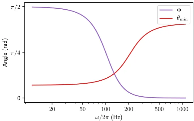
Defining Φ(ω) :=−arccot(K(ω)), and noting that K(ω)>0 and thus Φ(ω)∈ (−π/2,0), we have
1 =−p1 +K(ω)2sin Φ(ω), K(ω) = p1 +K(ω)2cos Φ(ω), (2.73)
so we can write
ˆ
Yπ/2(ω)− K(ω) ˆY0(ω) = p
1 +K(ω)2−sin Φ(ω) ˆY
π/2(ω)−cos Φ(ω) ˆY0(ω)
=p1 +K(ω)2(−cos Φ(ω) +isin Φ(ω))δˆb + (−cos Φ(ω)−isin Φ(ω))δˆb†
=−p1 +K(ω)2Yˆ
Φ(ω)(ω), (2.74)
and thus
h(ω) =−qSSQL(ω)
s
1 +K(ω)2 2K(ω) e
iβ(ω)ˆ
YΦ(ω)(ω). (2.75)
LetSb
θ(ω) denote the spectral density of theθ quadrature of the input fieldδˆb(as
in Eq. (2.61)). Using the fact that SSQL, Kand Φ are even functions of ω, andβ
is an odd function, we can thus write the noise spectrum for LIGO with input δˆb
as simply
SLIGOb (ω) = SSQL(ω)×1 2
1
K(ω) +K(ω)
SΦ(b ω)(ω)
=SLIGO(ω)SΦ(b ω)(ω). (2.76)