This is a repository copy of
Comparing robot controllers through system identification
.
White Rose Research Online URL for this paper:
http://eprints.whiterose.ac.uk/74561/
Monograph:
Nehmzow, U., Akanyeti, O., Iglesias, R. et al. (2 more authors) (2006) Comparing robot
controllers through system identification. Research Report. ACSE Research Report no.
921 . Automatic Control and Systems Engineering, University of Sheffield
[email protected]
https://eprints.whiterose.ac.uk/
Reuse
Unless indicated otherwise, fulltext items are protected by copyright with all rights reserved. The copyright
exception in section 29 of the Copyright, Designs and Patents Act 1988 allows the making of a single copy
solely for the purpose of non-commercial research or private study within the limits of fair dealing. The
publisher or other rights-holder may allow further reproduction and re-use of this version - refer to the White
Rose Research Online record for this item. Where records identify the publisher as the copyright holder,
users can verify any specific terms of use on the publisher’s website.
Takedown
If you consider content in White Rose Research Online to be in breach of UK law, please notify us by
Comparing Robot Controllers through System Identification
U Nehmzow
#, O Akanyeti
#, R Iglesias
#, T Kyriacou
#, S A Billings
#Dept Computer Science, University of Essex
Department of Automatic Control and Systems Engineering
The University of Sheffield, Sheffield, S1 3JD, UK
Research Report No. 921
Comparing Robot Controllers Through System
Identification
Ulrich Nehmzow1
, Otar Akanyeti1
, Roberto Iglesias2
, Theocharis Kyriacou1
and Steve Billings3
1
Dept. of Computer Science, University of Essex, UK.
2
Electronics and Computer Science, University of Santiago de Compostela, Spain.
3
Dept. of Automatic Control and Systems Engineering, University of Sheffield, UK.
Abstract. In the mobile robotics field, it is very common to find
dif-ferent control programs designed to achieve a particular robot task. Al-though there are many ways to evaluate these controllers qualitatively, there is a lack of formal methodology to compare them from a mathe-matical point of view.
In this paper we present a novel approach to compare robot control codes quantitatively based on system identification: Initially the transparent mathematical models of the controllers are obtained using the NARMAX system identification process. Then we use these models to analyse the general characteristics of the cotrollers from a mathematical point of view. In this way, we are able to compare different control programs objectively based on quantitative measures.
We demonstrate our approach by comparing two different robot con-trol programs, which were designed to drive the robot through door-like openings.
1
Introduction
In the mobile robotics field, it is very common to find different control pro-grams developed by different research groups to obtain the same behaviour in the robot. Generally, these control programs have been developed through an em-pirical trial-and-error process of iterative refinement, until the robot’s behaviour resembles the desired one to the desired degree of accuracy.
To date the main tendency to evaluate the developed controllers is based on qualitative analysis of the behaviour achieved by the robot rather than analytical principles. But with an increase in the number of controllers developed for the same task, the need to compare them based on quantitative measures becomes more important. So there is no doubt that analysing scientific questions like “What are the advantages and disadvantages of each controller?”, “Which one is more stable and efficient?”, “Will they work in completely different environments or crash even with slight modifications?” quantitatively, will contribute more information to the evaluation process of controllers.
answering these questions lies in the complex nature of today’s control programs which do not give enough information about how sensory perception contributes to a robot’s behaviour in a specific environment.
One possible way of comparing different robot control programs objectively is to evaluate their performances in the same test environments. However it is a cumbersome process for research groups to make experiments with other research group’s controllers because, due to the iterative refinement process of today’s robot programming techniques, generated controllers become highly robot-platform dependent, which makes it harder to utilise the solution across platforms or to be exchanged between different research groups.
In this paper, we present a novel approach to compare different robot con-trol programs, which were designed to obtain the same behaviour in the robot, from a mathematical point of view: first the controllers are identified by using non linear polynomials in such a way that the resulting transparent models can subsequently be used to control the movement of the robot. Then we use these transparent models to compare the controllers objectively based on quantitative measures.
2
Controller Identification
2.1 Motivation and Related Work
As a first stage to the evaluation process of control programs, we were interested to represent the controllers in the form of mathematical equations. The main benefits of “system identification” — in the sense of mathematical modelling — to the evaluation process can be summarised as follows:
1. Efficiency: The obtained models are generally non linear polynomials. They are fast in execution and they occupy little space in memory.
2. Transparency: Their transparent structure give us the flexibility to evaluate them from mathematical point of view.
3. Portability: Mathematical polynomials are universal. They can be exchanged between different research groups without any compatibility problem. Our models are obtained based on NARMAX (Nonlinear Auto-Regressive Moving Average model with eXogenous inputs) system identification [1]. This identification process has already been applied in modelling sensor-motor cou-plings of robot controllers [2, 4]. In [5], it has been shown how easy it is to ex-change the generated models between different research groups, using different robot platforms.
The system identification process can be divided into two stages: First the robot is driven by the robot controller which we want to identify. While the robot is moving, we log sensor and motor information to model the relationship between the robot’s sensor perception and motor responses.
After the identification of the controllers using mathematical models, it is relatively straightforward to evaluate the models using mathematical tools and to compare them quantitatively. The work presented in [3] gives examples of approaches can be used in the characterisation of these models.
2.2 NARMAX Modelling
The NARMAX modelling approach is a parameter estimation methodology for identifying the important model terms and associated parameters of unknown nonlinear dynamic systems. For multiple input, single output noiseless systems this model takes the form:
y(n) =f(u1(n), u1(n−1), u1(n−2),· · ·, u1(n−Nu), u1(n) 2
, u1(n−1) 2
, u1(n−2)
2
,· · ·, u1(n−Nu)
2
,· · ·, u1(n)l, u1(n−1)l, u1(n−2)l,· · ·,
u1(n−Nu)l, u2(n), u2(n−1), u2(n−2),· · ·, u2(n−Nu), u2(n) 2
, u2(n−1)
2
, u2(n−2) 2
,· · ·, u2(n−Nu)
2
,· · ·, u2(n)
l
, u2(n−1)
l , u2(n−2)
l
,· · ·, u2(n−Nu)l,· · ·, ud(n), ud(n−1), ud(n−2),· · ·,
ud(n−Nu), ud(n)
2
, ud(n−1)2, ud(n−2)2,· · ·, ud(n−Nu)
2
,· · ·,
ud(n)l, ud(n−1)l, ud(n−2)l,· · ·, ud(n−Nu)l, y(n−1), y(n−2),· · ·,
y(n−Ny), y(n−1)
2
, y(n−2)
2
,· · ·, y(n−Ny)
2
,· · ·, y(n−1)l,
y(n−2)l,· · ·, y(n−Ny)l)
wherey(n) andu(n) are the sampled output and input signals at timen
respec-tively,Ny and Nuare the regression orders of the output and input respectively and d is the input dimension.f() is a non-linear function, this is typically taken to be a polynomial or wavelet multi-resolution expansion of the arguments. The degreelof the polynomial is the highest sum of powers in any of its terms.
The NARMAX methodology breaks the modelling problem into the following steps:i) Structure detection, ii) parameter estimation, iii) model validation, iv) prediction and v) analysis.
Any data set that we intend to model is first split in two sets (usually of equal size). We call the first theestimation data set and it is used to determine the model structure and parameters. The remaining data set is called thevalidation data set and it is used to validate the model.
3
Experimental Setup: Door Traversal
One of the controllers is a “hard-wired laser controller” which maps the laser per-ception of the robot into action based on a behaviour based approach. For the second controller, the robot was driven manually by a human operator. During the first round of experiments, the translational velocity of robot was kept constant and both con-trollers drove the robot by changing its steering velocity at every instant. For each episode, we logged sensor information used by each controller and the angular velocity of the robot.
Then each controller was modelled by using non-linear polynomial functions (NAR-MAX) separately. The resulting two models identify the two robot controllers in terms of mathematical functions by relating robot perception to action. After having iden-tified models of robot controllers, we let the models themselves control the robot for confirmation that the models have captured the fundamental control strategy.
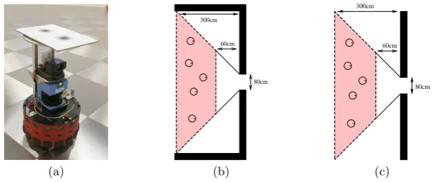
The models of the two differrent robot controllers were deliberately trained in dif-ferent environments (figure 1 (b,c)), with difdif-ferent translational velocities and difdif-ferent sensor information. Thus, we tried to simulate the differences which might exist be-tween different implementations of the same task.
All experiments were conducted with a Magellan Pro robot (figure 1 (a)) in the Robot Arena at Essex University. In each run, the trajectory of the robot was recorded by an overhead camera logging the coordinates of the robot approximately every 160 ms.
80cm 60cm 300cm
80cm 60cm 300cm
[image:6.595.150.466.358.490.2](a) (b) (c)
Fig. 1.The Magellan Pro robot used in the experiments (a). Training environments
for the “Hard-Wired Laser Controller” (b) and “Manual Control” (c). Environment (b) has extra walls on the wings of the door-like opening. The initial positions of the robot were within the shaded area indicated in each figure; door openings were twice the robot’s diameter (80cm).
3.1 Implementation 1: Hardwired Laser Control
The first control program used a hardwired control strategy that mapped laser percep-tion to steering speed of the robot.
robot was used as an input vector where laser measures were subsampled in 36 sectors by taking the median value of every 5 degree interval.
The model structure was of input lagNu= 0, output lagNy= 0, and degreel=
2. This produced a polynomial containing 84 terms. The final model equation for the angular velocityωis given in table 1.
ω= 0.574 + 0.045∗d1(t) + 0.001∗d6(t) + 0.032∗d7(t)−0.017∗d8(t)
+0.113∗d9(t)−0.099∗d10(t)−0.011∗d11(t)−0.006∗d12(t)−0.020∗d13(t)
+0.020∗d14(t)−0.015∗d15(t)−0.016∗d16(t)−0.046∗d20(t)−0.009∗d21(t)
+0.007∗d22(t)−0.035∗d23−0.017∗d24(t)−0.056∗d25(t) + 0.026∗d26(t)
+0.039∗d27(t)−0.003∗d28(t) + 0.044∗d29(t)−0.018∗d30(t)−0.144∗d31(t)
+0.001∗d32(t)−0.023∗d 2
1(t)−0.001∗d 2
6(t)−0.011∗d 2
7(t) + 0.003∗d 2 8(t)
−0.010∗d213(t)−0.001∗d 2
15(t)−0.005∗d 2
16(t)−0.001∗d 2 17(t)
−0.002∗d219(t) + 0.002∗d 2
20(t)−0.001∗d 2
21(t)−0.001∗d 2 22(t)
+0.002∗d223(t) + 0.002∗d 2
24(t) + 0.008∗d 2
25(t)−0.004∗d 2 27(t)
−0.001∗d228(t) + 0.019∗d 2
31(t)−0.001∗d 2
35(t) + 0.001∗d 2 36(t)
−0.001∗d1(t)∗d7(t)−0.001∗d1(t)∗d18(t) + 0.001∗d1(t)∗d20(t)
+0.003∗d1(t)∗d22(t) + 0.006∗d1(t)∗d23(t)−0.003∗d1(t)∗d25(t)
−0.001∗d1(t)∗d32(t) + 0.003∗d1(t)∗d33(t) + 0.007∗d1(t)∗d34(t)
−0.002∗d1(t)∗d36(t) + 0.003∗d7(t)∗d16(t)−0.001∗d8(t)∗d10(t)
−0.006∗d9(t)∗d14(t)−0.003∗d9(t)∗d17(t)−0.009∗d9(t)∗d18(t)
−0.002∗d9(t)∗d28(t) + 0.013∗d10(t)∗d13(t)−0.002∗d11(t)∗d16(t)
+0.004∗d11(t)∗d18(t)−0.001∗d12(t)∗d15(t) + 0.001∗d12(t)∗d16(t)
+0.002∗d12(t)∗d18(t) + 0.002∗d13(t)∗d15(t) + 0.011∗d13(t)∗d16(t)
−0.003∗d14(t)∗d16(t) + 0.002∗d14(t)∗d23(t) + 0.001∗d14(t)∗d36(t)
+0.002∗d15(t)∗d21(t) + 0.003∗d16(t)∗d19(t) + 0.002∗d16(t)∗d25(t)
+0.002∗d17(t)∗d28(t) + 0.001∗d18(t)∗d31(t) + 0.001∗d20(t)∗d21(t)
+0.002∗d20(t)∗d28(t) + 0.003∗d20(t)∗d31(t)−0.004∗d21(t)∗d26(t)
+0.005∗d21(t)∗d30(t)−0.005∗d25(t)∗d29(t)
Table 1.Model 1: NARMAX model of the angular velocity ωas a function of laser
perception for the “hard-wired laser controller”.d1,· · ·, d29are laser bins, coarse coded
by taking the median value every 5 degree interval.
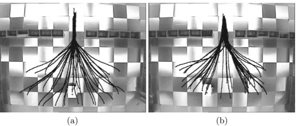
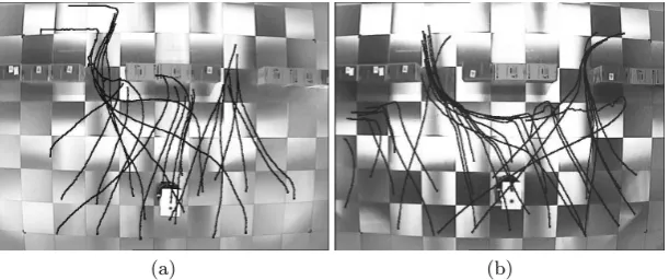
Figure 2 shows the trajectories of the robot under the control of the hard-wired laser controller and its NARMAX model respectively. The robot was started with 36 different initial positions passing through the door-like gap successfully in each episode.
3.2 Implementation 2: Manual Control
The second control strategy we used, to contrast with the “hard-wired laser controller” was to drive the robot through the opening manually.
(a) (b)
Fig. 2.Robot trajectories under control by the original “Hard-wired Laser Controller”
(a) and under control by its model, “model 1” (b). Note that side walls of the environ-ment can not be seen in the figures because they were outside the field of view of the camera.
The model structure again was of input lagNu= 0, output lagNy= 0, and degree l = 2. The produced polynomial contained 35 terms. The final model equation for angular velocityωis given in table 2.
ω(t) = 0.010−1.633∗d′1(t)−2.482∗d′2(t) + 0.171∗d′3(t) + 0.977∗d′4(t)
−1.033∗d′5(t) + 1.947∗d′6(t) + 0.331∗s′13(t)−1.257∗s′15(t) + 12.639∗d
′2 1 (t)
+16.474∗d′22(t) + 28.175∗s
′2
15(t) + 80.032∗s
′2
16(t) + 14.403∗d′1(t)∗d′3(t)
−209.752∗d′1(t)∗d′5(t)−5.583∗d′1(t)∗d′6(t) + 178.641∗d′1(t)∗s′11(t)
−126.311∗d′1(t)∗s′16(t) + 1.662∗d′2(t)∗d′3(t) + 225.522∗d′2(t)∗d′5(t)
−173.078∗d′2(t)∗s′11(t) + 25.348∗d′3(t)∗s′12(t)−24.699∗d′3(t)∗s′15(t)
+100.242∗d′4(t)∗d6′(t)−17.954∗d′4(t)∗s′12(t)−3.886∗d′4(t)∗s′15(t)
−173.255∗d′5(t)∗s′11(t) + 40.926∗d′5(t)∗s′15(t)−73.090∗d′5(t)∗s′16(t)
−144.247∗d′6(t)∗s′12(t)−57.092∗d′6(t)∗s′13(t)) + 36.413∗d′6(t)∗s′14(t)
−55.085∗s′11(t)∗s′14(t) + 28.286∗s′12(t)∗s′15(t)−11.211∗s′14(t)∗s′16(t)
Table 2.Model 2: NARMAX model of the angular velocityωas a function of sensor
perception for the door traversal behaviour under manual control.s10,· · ·, s16 are the
inverted and normalised sonar readings (s′
i= (1/si−0.25)/19.75), whiled1,· · ·, d6are
the inverted and normalised laser binsd′
i= (1/di−0.12)/19.88. Taken from [4].
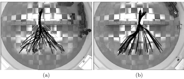
Figure 3 shows the trajectories of the robot under the control of human operator and its NARMAX model respectively. The robot was started with 41 different initial positions and it has passed through the door-like gap successfully in each episode.
4
Comparison of the Two Models
(a) (b)
Fig. 3.Robot Trajectories under under “manual control” (a) and under control of its
model, “model 2” (b). Taken from [4].
to see that “Model 1” has significantly more terms (83) than “Model 2” (35). Another remarkable observation is that “Model 2” uses only information from sensors found on the right side of the robot.
So we have two non-linear polynomial functions, using different sensor perception, running with different translational velocities, but aiming to solve the same problem: door traversal. This section shows several ways of how NARMAX models can be used to analyse these controllers qualitatively as well as quantitatively, in order to decide if they are actually the same in terms of robot-environment interaction or not.
First, we tested the controllers in four different environments (figure 4) to reveal differences in the behaviours of the robot controlled by the two models. During the experiments, in order to avoid constant errors related to the robot itself, a randomisa-tion process was used: both models were uploaded to the robot together and for each episode the robot picked one of them randomly.
In the first scenario (figure 4 (1)), the robot was driven by “Model 1” in the training environment of “Model 2”. In this way, we hoped to observe how slight modifications in the test environment, compared to “Model 1” train environment, can effect the behaviour of the robot.
Then the two controllers were tested in a completely different environment, where two door-like openings with equal width were presented at the same time (figure 4 (2)). This demonstrated how each opening interfered with the robot’s behaviour. It also revealed the dominant sensors, influencing the behaviour of the robot.
In the third and fourth scenarios (figure 4 (3) and (4)) , we tried to measure the effect of a gap found in an environment on the robot behaviour. We assumed that in this application openings would be the dominant environmental factors in robot-environment interaction. Therefore the models were tested first in a completely closed environment without any gaps, then we tried to observe the difference in robot behaviours for each model separately by introducing an opening to the environment.
4.1 Qualitative Comparison
80cm
80cm
80cm
80cm
[image:10.595.138.451.114.234.2](1) (2) (3) (4)
Fig. 4.Four different test environments used to compare the two models qualitatively.
1) Single-door test scenario, 2) Double-door test scenario, 3) Completely-enclosed test scenario, 4) Enclosure with a single door. The initial positions of the robot are within the shaded area indicated in each figure. All openings found in the environment had a width of two robot diameters (80cm).
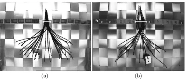
approaching to the door-like opening so it was easier for robot to center itself while passing through the gap.
(a) (b)
Fig. 5.Robot trajectories under the control of “Model 1” in the training environment
of “Model 1” (a), and in the training environment of “Model 2” (b). The arrows in both figures indicate how much the robot deviated from the centre point of the opening while passing through it. Note that side walls of the environment in (A) can not be seen in the figure because of the limited range of camera view.
For the double-door test scenario, it is interesting to see how two gaps interfere with each other for the behaviour of robot under the control of “Model 1”. If the robot was started from the middle region between two gaps, it generally bumps into the wall without turning towards any of the gaps. If the robot points to one of the gaps initially, it is attracted towards it but the other gap still effects the behaviour and the robot cannot center itself enough to pass through the gap (figure 6 (a)).
[image:10.595.157.463.362.492.2]double-door environments. “Model 2” uses sensors only from one side of the robot, so basically if it detects the gap found on the right side of itself, it passes through it. If it doesn’t, it automatically turns to the left and finds the other gap and follows it.
[image:11.595.156.462.172.300.2](a) (b)
Fig. 6. Robot Trajectories in the “double door” test scenario under the control of
“Model 1” (a), and controlled by “Model 2” (b).
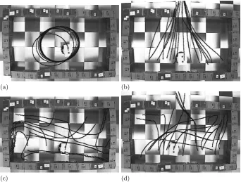
In the completely-enclosed environment, “Model 1” turned the robot constantly to the left. Figure 7 (a) shows a sample trajectory of robot under he control of “Model 1”. When we introduce a gap to the environment, we observed that gap has the dominating effect on the controller behaviour. Although the model can not pass through the gap successfully in every trial, we still observe a general flow in the behaviour of robot towards the gap (figure 7 (b)).
Finally, “Model 2” showed very unstable characteristics in the last two environ-ments. When we look at the trajectories closely we observe oscillations in the robot’s behaviour, especially when the robot is facing the corners from a close distance. The overall model generally looks like a right wall follower when the robot is distant from the corners. As it comes closer, the variation in angular velocity of the robot increases and it bumps into the corners (figure 7 (c)). Also we can say that for “Model 2”, the influence of the gap on the robot behaviour is not as big as the influence for “Model 1” (figure 7 (d)).
4.2 Quantitative Comparison
When we look at the behaviours of the robot qualitatively in different test environ-ments, we see that the responses of the two models differ. We also observe that both models have poor “generalisation” ability in the sense of passing through door like openings successfully in different environments.
In this section, we extended our work by comparing the two models quantitatively, based on a “hardware in the loop simulation” process: We fed the two models with same sensory perception of the robot, taken from the real test environments, and then compare the consequent outputs of the models in order to see if there is a correlation between the responses of the two models.
(a) (b)
[image:12.595.136.479.116.375.2](c) (d)
Fig. 7.Robot trajectories under control of “Model 1”in in the “Completely enclosed
environment” (a) and when an opening is introduced to the enclosed environment (b). Robot trajectories under control of “Model 2” in the “Completely enclosed environ-ment” (c), and when an opening is introduced to the enclosed environment (d).
resulting angular velocity by using the two models. As an example, figure 8(b) shows the steering velocity which the robot would attain along the sample trajectory (figure 8(a)) at every instantt, when the robot is driven by the two models individually.
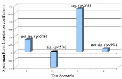
Then we computed Spearman rank correlation coefficients [6] between the two model’s steering velocity vectors for each test environment individually. As can be seen in figure 9, test results show that there is no significant correlation between the two model’s responses for “single door” and “encloseure with a single door” test scenarios. For the other two scenarios, again the correlation between the two model’s responses is very low, indicating substantial differences between the two models.
5
Summary and Conclusion
(a) (b)
Fig. 8. Trajectory along which sensor data for “hardware in the loop” simulation
was taken (a), and steering velocity graphs of both models for the given trajectory (b). There is no significant correlation between the two model’s angular velocities (rS=0.078, not sig.,p>5%).
Fig. 9. Spearman rank correlation coefficients between the two model’s
[image:13.595.209.405.439.566.2]In order to compare these two behaviours, we “identified” both behaviours, that is, we determined transparent, analysable nonlinear polynomial mappings between sensor perception and motor response, and subsequently compared the two models with each other. Such transfer to a common descriptor of behaviour has a number of advantages: in some cases, no explicit representation of the control strategy is available at all (e.g. under manual control), code can very easily be transfered between different robot platforms
Furthermore, once transparent mathematical models of sensor motor behaviour are available, they can be analysed quantitatively. In the experiments presented in this paper, we used a hardware-in-the-loop simulation to demonstrate that the hardwired and the manual control strategy differ from each other significantly. Other analysis methods include analysing the models’ spectra, applying stability analysis [7], or using sensitivity analysis [8–10]. Such detailed mathematical analysis of the polynomials is part of ongoing research at the universities of Sheffield and Essex.
Acknowledgements
The authors would like to thank Hugo Vieira Neto for his contributions to the prepara-tion of this paper. The authors also thank to the following instituprepara-tions for their support: The RobotMODIC project is supported by the Engineering and Physical Sciences Re-search Council under grant GR/S30955/01. Roberto Iglesias is supported through the research grants PGIDIT04TIC206011PR, TIC2003-09400-C04-03 and TIN2005-03844.
References
[1] Korenberg, M., Billings, S. A., Liu, Y. P., and Mcllroy, P. J., Orthogonal Parameter Estimation Algorithm for Non-Linear Stochastic Systems,Int. J. Control, 1998, vol 48(1):193-210.
[2] Iglesias, R., Kyriacou, T., Nehmzow, U., and Billings, S. A., Task Identification and Characterisation in Mobile Robotics,Proc. ”Towards Autonomous Robotic Systems”,
TAROS, Essex 2004.
[3] Iglesias, R., Kyriacou, T., Nehmzow, U., and Billings, S. A., Modelling and char-acterisation of a mobile robot’s operation,Proc. ”CAEPIA 2005, 11th Conference of the Spanish association for Artificial Intelligence”,Santiago De Compostela 2005. [4] Iglesias, R., Nehmzow, U., Kyriacou, T., and Billings, S. A., Programming Through
System Identification and Training,Proc. European Conference on Mobile Robotics, Ancona 2005.
[5] Kyriacou, T., Nehmzow, U., Iglesias, R., and Billings, S. A., Cross-Platform Pro-gramming Through System Identification,Proc. ”Towards Autonomous Robotic Sys-tems”, TAROS, London 2005.
[6] Barnard, C., Gilber, F., and McGregor, P.,Asking questions in Biology, key Skills for Practical Assessments and Project Work, Pearson Education Limited, 2001. [7] P.C. Dorf and R.H. Bishop, Modern Control Systems; Addison Wesley 1995 [8] Max D. Morris, Factorial sampling plans for preliminary computational
experi-ments,Technometrics, v.33 n.2, p.161-174, May 1991.
[9] A. Saltelli, K. Chan and E.M. Scott,Sensitivity Analysis, John Wiley 2000 [10] I.M. Sobol, Sensitivity Estimates for Nonlinear Mathematical Models,