City, University of London Institutional Repository
Citation
:
Lee, Y. K., Mammen, E., Nielsen, J. P. & Park, B. U. (2017). Operational time and in-sample density forecasting. Annals of Statistics, 45(3), pp. 1312-1341. doi:10.1214/16-AOS1486
This is the published version of the paper.
This version of the publication may differ from the final published
version.
Permanent repository link: http://openaccess.city.ac.uk/15176/
Link to published version
:
http://dx.doi.org/10.1214/16-AOS1486Copyright and reuse:
City Research Online aims to make research
outputs of City, University of London available to a wider audience.
Copyright and Moral Rights remain with the author(s) and/or copyright
holders. URLs from City Research Online may be freely distributed and
linked to.
City Research Online: http://openaccess.city.ac.uk/ [email protected]
2017, Vol. 45, No. 3, 1312–1341 DOI:10.1214/16-AOS1486
©Institute of Mathematical Statistics, 2017
OPERATIONAL TIME AND IN-SAMPLE DENSITY FORECASTING
BYYOUNG K. LEE1,∗, ENNOMAMMEN2,†, JENSP. NIELSEN3,‡ANDBYEONGU. PARK4,§
Kangwon National University∗, Universität Heidelberg and Higher School of Economics†, Cass Business School, City University London‡
and Seoul National University§
In this paper, we consider a new structural model for in-sample density forecasting. In-sample density forecasting is to estimate a structured density on a region where data are observed and then reuse the estimated structured density on some region where data are not observed. Our structural assump-tion is that the density is a product of one-dimensional funcassump-tions with one function sitting on the scale of a transformed space of observations. The transformation involves another unknown one-dimensional function, so that our model is formulated via a known smooth function of three underlying unknown one-dimensional functions. We present an innovative way of esti-mating the one-dimensional functions and show that all the estimators of the three components achieve the optimal one-dimensional rate of convergence. We illustrate how one can use our approach by analyzing a real dataset, and also verify the tractable finite sample performance of the method via a simu-lation study.
1. Introduction. In-sample forecasting is a recently introduced class of fore-casting methods based on structured nonparametric models. The idea is that obser-vations might fall in some set, sayS, inR2 and thatScan be written as the union of two subsetsS1andS2, whereS1is the set of observed observations andS2is the
set of future observations whose distribution is the target for forecasting. In-sample density forecasting assumes that the density restricted to S1 or to S2 can be
de-scribed by the same one-dimensional nonparametric functions. This assumptions leads to the convenient forecasting strategy of estimating the structured density on the observed data inS1 and then simply reusing the nonparametrically estimated
Received July 2015; revised June 2016.
1Supported by the National Research Foundation of Korea (NRF) grant funded by the Korea
gov-ernment (MSIP) (NRF-2015R1A2A2A01005039).
2Supported by Deutsche Forschungsgemeinschaft through the Research Training Group RTG 1953
and by the Government of the Russian Federation within the framework of the implementation of the Global Competitiveness Program of the National Research University Higher School of Economics.
3Supported by the Institute and Faculty of Actuaries, London.
4Supported by the National Research Foundation of Korea (NRF) grant funded by the Korea
gov-ernment (MSIP) (NRF-2015R1A2A1A05001753).
MSC2010 subject classifications.Primary 62G07; secondary 62G20.
Key words and phrases.Density estimation, kernel smoothing, backfitting, chain Ladder.
one-dimensional components while estimating the density onS2. The strategy may
be put into practice by structuring the density in such a way that all components of the structured density are estimable with the observations inS1. With this strategy,
forecasting can be performed without extrapolation of parameters. This is likely to lead to more robust forecasting, because extrapolated parameters are often volatile. For time series extrapolation in particular, seeLee and Carter(1992), for example.
Lee et al.(2015) andMammen, Martínez Miranda and Nielsen(2015) consid-ered the perhaps simplest possible in-sample forecaster, where the joint density
phas a multiplicative structurep(x, y)=f1(x)f2(y)for some unknown
univari-ate functionsfj withS1= {(x, y):x≥0, y≥0, x+y≤t0}. In this setting, pis
the joint density of two random variablesX andY, whereX represents the start of something and Y is the development to some event from this starting point. These variables are observed only if the event occurs by a fixed calendar timet0.
Thus,f1(x)measures how many individuals are exposed or under risk andf2(y)
represents duration or survival. The multiplicative form means that survival or du-ration has the same distribution independent ofX. As was pointed out inLee et al.
(2015) andMammen, Martínez Miranda and Nielsen(2015), this is a continuous type in-sample forecaster that extends classical actuarial and mortality forecast-ing methodologies based on multiplicative Poisson models beforecast-ing used every day in virtually all nonlife insurance companies around the world. In a nonparametric universe, the estimators resulting from the multiplicative Poisson models are struc-tured histograms.Martínez-Miranda et al.(2013) showed the link between actuar-ial parametric chain ladder-type models [Kuang, Nielsen and Nielsen(2009)] and structured smoothing as considered in this paper.
The multiplicative structure f1(x)f2(y) may be too simple for many settings.
Nevertheless, the multiplicative model can be used as a baseline for more sophis-ticated models that deviate from this simple structure. This paper illustrates how powerful in-sample forecasting is when formulating, interpreting and analysing extensions of the simple multiplicative model. Actuaries have long tried to intro-duce the concept of operational time in the claims reserving modelling. The phrase “operational time” is taken from the literature of Poisson processes. When trans-forming the time axis with its operational time, an inhomogeneous Poisson process is transformed to a homogenous one; seeMikosch(2009) among many others. In the claims modelling framework, actuaries have been concerned about adjusting for changes in the speed of claims finalization over time. Many actuarial confer-ence proceeding papers have been devoted to this topic and still are to this day. However, operational time or speed of claims finalization only had a short blos-soming in the more formal academic actuarial literature; seeReid(1978),Taylor
This paper introduces operational time to a general class of multiplicative mod-els including actuarial, demographic and labour market applications taking ad-vantage of the general in-sample forecasting formulation. We refer toLee et al.
(2015), Mammen, Martínez Miranda and Nielsen (2015) and Wilke (2016) for practical illustrations of multiplicative In-sample forecasting in actuarial science, demographics and the labour market. An alternative to operational time could be to add a calendar effect to the multiplicative model. While calendar effects are popular to talk about in actuarial science, they cause a number of difficulties, the most serious being the identifiability issue that some arbitrary linear trends can be added to or subtracted from the underlying model without changing the underlying model; seeKuang, Nielsen and Nielsen(2008a,2008b,2011). While the latter of these three papers does suggest practical implementation of identified forecasting procedures using calendar effects, there is still considerable uncertainty on how to forecast calendar effects in practice in the simple multiplicative forecasting model. Our Operational Time In-Sample Forecaster does not have any of these practical problems. It is immediate to construct a practical forecaster based on the opera-tional time extension of the simple multiplicative In-Sample Forecaster.
In this paper, we consider a transformation, sayφ, and a density model given by
p(x, y)=f1(x)f2(yφ(x))onS1. Our method and theory apply to a general type
of support setS1. The Operational Time In-Sample Forecaster can be understood
as a structured model formulated in a density framework rather than in the regres-sion framework considered inMammen and Nielsen(2003). The model is formu-lated via a known smooth function of three one-dimensional unknown functions
φ, f1 andf2. The estimation ofφ, as discussed in Section3, involves the
estima-tion of the partial derivatives of the two-dimensional joint density funcestima-tion p by kernel smoothing. A naive application of the standard theory of kernel smoothing to the problem renders only a sub-optimal rate of convergence for the estimator ofφ. Based on an innovative asymptotic analysis, we show that our estimator ofφ
achieves the optimal one-dimensional rate. Using this result, we also establish that the component functionsfj can be estimated with the optimal univariate rate.
There is a close relation between the multiplicative density model and the ad-ditive regression model. Thus, our approach may be extended to fundamental structured regression models studied in Jiang, Fan and Fan(2010),Yu, Park and Mammen(2008), Lee, Mammen and Park (2010,2012),Zhang, Park and Wang
(2013) among others. The multiplicative model with operational time corresponds to nonparametric regression models of the formZ=m1(X)+m2(Y φ(X))+εor Z=m1(X)+m2(Y+φ(X))+ε. The latter model is related to the nonparametric
neural network models studied inHorowitz and Mammen(2007); see also recent work on composite function models byJuditsky, Lepski and Tsybakov(2009) and
Baraud and Birgé(2014).
happened and on a retrospective observation of the onset of these events. There-fore, there needs to be a lot less data to keep track of. For example, in-sample fore-casting requires only keeping track of actual deaths of AIDS and retrospectively observed onset of AIDS, while most of survival analysis techniques need full fol-low up of how many individuals are under risk at any time (exposure), in addition to actual deaths of AIDS. The reason that in-sample forecasting needs fewer data requirements is that it estimates from data the equivalent of exposure in survival analysis. Our model is in some way related to accelerated failure time models. If one assumes that exposure is fully known and that one has only the componentsf2
andφin the model, then our model compares to an accelerated failure time model with X being a covariate; see Example VII 6.3 inAndersen et al. (1993). How-ever, there are some differences. First of all, our approach is fully nonparametric. Second, our data are right truncated. Thus, exposure is not observed and it is only indirectly represented in our model via the componentf1and estimated from the
data. We therefore note that survival analysis techniques are not directly applicable in our model or in the application discussed in Section7in particular.
2. The model. We observe a random sample {(Xi, Yi):1≤i≤n} from a
densitypsupported on a subsetIof the unit rectangle[0,1]2. The densityp(x, y)
of(Xi, Yi)is a multiplicative function
(2.1) p(x, y)=f1(x)f2
yφ(x), (x, y)∈I,
wheref1,f2 andφ are unknown nonnegative functions bounded away from zero
on their supports. We assume thatf1 andφ are supported on[0,1]. We begin by
considering the triangular support setI= {(x, y):0≤x, y≤1, x+y≤1} of a rectangle[0,1]2since the main idea of our approach can be best conveyed through the simple case. We discuss the method and theory for a general type of support set in Section5.
We start with the identification of the functionφ in the model (2.1). The idea is also used for nonparametric estimation of the function, which we detail in the next section. Note that
∂
∂x logp(x, y)= f1(x) f1(x) +
f2(yφ(x)) f2(yφ(x))
yφ(x),
∂
∂y logp(x, y)=
f2(yφ(x)) f2(yφ(x))
φ(x).
To represent φ in terms of the two partial derivatives, we think of a suitable contrast function w(·;x):R→R for each x ∈ [0,1), having the property that
1−x
0 w(y;x) dy=0. Then we have
1−x
0
∂
∂xlogp(x, y)
w(y;x) dy=A(x)φ(x),
1−x
0
∂
∂y logp(x, y)
yw(y;x) dy=A(x)φ(x),
where
A(x)=
1−x
0
f2(yφ(x)) f2(yφ(x))
yw(y;x) dy.
IfA(x)=0 for allx∈ [0,1), then we get
φ(x) φ(x) =
1−x
0 (
∂
∂xlogp(x, y))w(y;x) dy
1−x
0 (∂y∂ logp(x, y))yw(y;x) dy .
For the contrast functionw, we take
w(y;x)=y ∂
∂y logp(x, y)−
1 1−x
1−x
0 y
∂
∂y logp(x, y) dy.
Note thaty∂logp(x, y)/∂y=yφ(x)f2(yφ(x))/f2(yφ(x))is actually a function
ofyφ(x), and that with the choice ofwwe get
1 1−x
1−x
0
∂
∂ylogp(x, y)
yw(y;x) dy
= 1
τ (x)
τ (x)
0
z·f
2(z) f2(z)
2 dz− 1 τ (x) τ (x) 0
z·f
2(z) f2(z)
dz
2
,
whereτ (x)=(1−x)φ(x). Thus,A(x) >0 ifzf2(z)/f2(z)is not a function that is
constant a.e. on(0, τ (x)). Now, forx0fixed,
lnφ(x)/φ(x0)
= x
x0
φ(u) φ(u) du=
x
x0
1−u
0 (
∂
∂ulogp(u, y))w(y;u) dy
1−u
We choosex0=0 and take the normalizationφ(0)=1. Forj, k=0,1,2, define
(2.2) Gj k(x)=
1 1−x
1−x
0
∂
∂xlogp(x, y)
j
y ∂
∂ylogp(x, y)
k
dy.
Then we get
(2.3) φ(x)=exp
x
0
G11(u)−G10(u)G01(u) G02(u)−G01(u)2
du .
To assure thatA(x) >0 for anyx∈ [0,1), we make the following assumption:
(A1) For any smallc >0, zf2(z)/f2(z)is not a function that is constant a.e. on (0, c).
Note that assumption (A1) concerns the behavior of the functionzf2(z)/f (z)near
z=0 only, since a function is not constant on(0, c1)if the function is not on(0, c2)
forc2< c1. The assumption is implied by the simpler one that there exists a small c0>0 such thatzf2(z)/f (z)is strictly monotone on(0, c0), or that its derivative
is not zero atz=0 in case it is continuously differentiable.
Next, we discuss the identifiability of the component functionsf1 andf2. The
following arguments are based on the identifiability of φ, which we have just proved. The two component functionsf1andf2are identifiable only up to a
mul-tiplicative constant. Hence, we put the constraint on the first component that
(2.4)
1
0
f1(x) dx=1.
Letμ1(x)=logf1(x)andμ2(z)=logf2(z). Suppose thatμ1(x)+μ2(yφ(x))=
0 for all(x, y)∈I. By differentiating both sides with respect toy, we get
φ(x)μ2yφ(x)=0.
Since we assume thatφ(x) >0 for allx∈ [0,1], this impliesμ2(yφ(x))=0 for all(x, y)∈I. Thus,μ2 is constant on its domain, so isμ1. Due to the constraint
(2.4), we haveμ1≡0 on[0,1]so thatμ2≡0 on its domain as well.
THEOREM1. Assume that the two component functionsfj and the time trans-formationφ in the model(2.1) are differentiable,nonnegative and bounded away from zero on their supports.Assume also that(A1)holds.Then the three functions φ,f1andf2are identifiable under the constraint(2.4).
performance at the boundary area ofI in the estimation of the partial derivatives. Indeed, in our preliminary simulation study we found that local linear smoothing produced quite bad estimates of the first partial derivatives.
To define the estimator ofφbased on local quadratic smoothing, let
a(u, v;x, y)=1, (u−x)/ h1, (v−y)/ h2, (u−x)2/ h21, (u−x)(v−y)/ h1h2, (v−y)2/ h22
,
A(x, y)=
Ia(u, v;x, y)a(u, v;x, y) h−1
1 h− 1 2 K
u−x
h1
K
v−y
h2
du dv,
where(h1, h2)is the bandwidth vector andKis a symmetric univariate probability
density function. Also, define
ˆ
b(x, y)=n−1 n
i=1
a(Xi, Yi;x, y)h−11h− 1 2 K
X
i−x h1
K
Y
i−y h2
.
The local quadratic density estimators of p(x, y), ∂x∂ p(x, y) and ∂y∂ p(x, y), re-spectively, are then defined byηˆ00(x, y),ηˆ10(x, y)/ h1 andηˆ01(x, y)/ h2,
respec-tively, where
(3.1) (ηˆ00,ηˆ10,ηˆ01,ηˆ20,ηˆ11,ηˆ02)=A−1bˆ.
The above estimators of the joint densitypand its partial derivatives are similar in spirit to the local linear density estimators studied inCheng(1997). Putting these into formula (2.2), we get the estimatorsGˆj k(x)ofGj k(x), and thus the estimator
ofφ defined by
(3.2) φ(x)ˆ =exp
x
0 ˆ
G11(u)− ˆG10(u)Gˆ01(u) ˆ
G02(u)− ˆG01(u)2
du .
The convergence rate of the estimatorφˆ depends on those of the estimatorsηˆj k
of the joint density and its partial derivatives. For simplicity of presentation we write
pj k(x, y)= ∂j+k
∂xj∂ykp(x, y).
If p is twice partially continuously differentiable, then from an expansion of
p(u, v) for (u, v) around (x, y) one gets that Eηˆj k(x, y)− hj1hk2pj k(x, y) = o(h21 +h22) for (j, k) with 0≤ j, k ≤ 1 and j +k ≤ 1. Furthermore, one has ηˆj k(x, y) − Eηˆj k(x, y) =Op(n−1/2h−11/2h−
1/2
2 ); see Ruppert and Wand
(1994) or Fan, Heckman and Wand (1995) among others. These imply that the estimators of the first-order partial derivatives have the convergence rate
h2). Note that the estimatorφ(x)ˆ involves two integrations of the estimators of the
first-order partial derivatives, one for each coordinate; see the definitions (2.2) and (3.2). In the standard kernel smoothing theory, it is well known that a nontrivial integration of a kernel estimator makes the stochastic part get smaller by an or-der ofh1/2, wherehis the size of the bandwidth that is used for local smoothing along the line of the integration. This is mainly because the “local average” turns into a “global average” along the lines of the integration; seeMammen, Park and Schienle(2014), for example. For the bias term, an integration does not reduce the order of magnitude in general, however. A direct application of this standard theory toφ(x)ˆ would give the rateOp(n−1/2min{h1, h2}−1)+op(max{h1, h2}).
One may improve the rate for the bias part to Op(max{h1, h2}2) if one assumes
three times partial differentiability, which would lead to the two-dimensional rate
n−1/3at best by choosingh1∼h2∼n−1/6.
In the theorem below, however, we show that our estimatorφˆ achieves the uni-variate rate of convergence n−2/5 under the condition that p is twice partially continuously differentiable. Before we state the theorem, here we give an intuition behind and heuristic argument for the surprising results. Letm2(u)=logf2(eu)
andm3(u)=logφ(u), wheref2 is the second component function in our model
(2.1). For an arbitrarily small constant >0, define a bivariate functionF by
(3.3) F(x, t)=
t+
t
logpx, ezdz−
t
t−
logpx, ezdz
on{(x, t):0≤x <1, t≤log(1−x)−}. ThenF may be expressed in terms of
a univariate function andφ. Indeed, lettingH(t)=
0[m2(z+t)−m2(z−+ t)]dz, we get
F(x, t)=
0
m2
z+t+m3(x)
−m2
z−+t+m3(x)
dz
=H
t+m3(x)
.
Recall our normalization φ(0)= 1 for φ, so that m3(0) =0. Thus, for t ≤
logτ (x)−we get
(3.4) F
x,−m3(x)+t
=H(t)=F(0, t).
From the definition of F at (3.3) we note that F may be estimated with the
univariate rate, because of the integration. Now, due to (3.4) one may identify
m3, thus φ, by identifying F, provided that, for any x∈ [0,1), one finds t0<
logτ (x)−such that∂F(x, t)/∂t is not zero att= −m3(x)+t0. The latter also
means thatm3 can be estimated with the same accuracy asF. The condition on ∂F(x, t)/∂t is implied by the assumption (A1). To see this, we note that
∂
∂tF(x, t)
t=−m3(x)+t0
Observing that m2(t) =etf2(et)/f2(et), the assumption (A1) is equivalent to
the condition that, for any C >0, m2 is not a function that is constant a.e. on
(−∞,−C). Thus, (A1) implies that, for anyC >0, there existst0<−C−such
thatH(t0)=0.
We now state our theorem for the rate of φ(x)ˆ . Below, we give a pointwise convergence rate forx ∈ [0,1), excluding the point x =1. Also, we present the rates for the integrated squared and the uniform errors on an interval [0,1−]
for an arbitrarily small >0. The reason we exclude the point x=1 is that the marginal density ofXvanishes atx=1 even though the joint densityf is bounded away from zero on its support. This is due to the triangular shape of the support setI. Thus, the consistent estimation ofφ(x) asx approaches to the end point 1 is not possible. We make the following additional assumptions:
(A2) The joint density function p is twice partially continuously differentiable and bounded away from zero;
(A3) The kernelK is supported on[−1,1], symmetric and Lipschitz continuous; (A4) The bandwidthsh1andh2are of ordern−1/5.
THEOREM2. Assume that the conditions of Theorem1and conditions(A2)–
(A4)are satisfied.Then we get forx∈ [0,1)that
(3.5) φ(x)ˆ −φ(x)=Op
n−2/5.
Furthermore,for an arbitrarily small >0,it holds that
1−
0
ˆ
φ(x)−φ(x)2dx=Op
n−4/5,
(3.6)
sup
x∈[0,1−]
φ(x)ˆ −φ(x)=Op
n−2/5
logn.
(3.7)
In the proof of Theorem2given in the Appendix, one sees thatφ(x)ˆ is not a local smoother. If one looks at the term J1(x) that is discussed at the end of the
proof, one finds that this quadratic form is of orderOp(n−2/5)and not negligible
in the first order. By definition all observations(Xi, Yi)enterJ1(x) with weights
of the same magnitude. Thus, this term does not rely only on local information. The same holds for φ(x)ˆ . It is calculated using all observations, not only those
(Xi, Yi) withXi in a shrinking neighborhood ofx. This makesφˆ quite different
from a kernel smoother.
4. Estimation of component functions. Suppose we know the true time transformation φ. Then we would convert the dataset (Xi, Yi) to (Xi, Zi) with Zi =Yiφ(Xi), and estimate the component functions f1 and f2 from the
the model (2.1) reduces to
(4.1) p
x, z φ(x)
=f1(x)f2(z).
Recall that we take the normalizationφ(0)=1. This means that time runs as real time at the starting point, and that the set{(u, vφ(u)):(u, v)∈I}includes the two edge points(0,1)and(1,0)of the triangleI.
For the estimation of the component functions f1 and f2 at points x and z,
respectively, we need sufficient data Xi and Zi around x and z. We
esti-mate f1 and f2 on intervals where the marginal densities of Xi and Zi,
re-spectively, are bounded away from zero. Note that the marginal density of Xi
at x and that of Zi at z are given by
(1−x)φ (x)
0 p(x, z/φ(x))/φ(x) dz and
x:τ (x)≥zp(x, z/φ(x))/φ(x) dx, respectively, where τ defined by τ (x)=(1− x)φ(x). We assume:
(A5) τ is strictly decreasing.
Condition (A5) simplifies the description of the method and the presentation of its theory. In this case{x∈ [0,1] :τ (x)≥z} = [0, τ−1(z)], and τ−1(z)=0 holds only for z=1. The method we describe below and its theory are based on this condition onτ. We discuss a general case at the end of this section.
The marginal density function ofXiequals zero atx=1 and that ofZiis zero
atz=1, even if the joint densitypis bounded away from zero on its support. For a set of(x, z)where we estimate the component functionsf1andf2, we take
I≡u, vφ(u):u≤1−, vφ(u)≤1−, (u, v)∈I
=(u, w):0≤u≤1−,0≤w≤(1−)∧τ (u)
(4.2)
for an arbitrarily small >0. The projections of the setI ontox- andz-axis equal
[0,1−]. Thus, we estimate both f1 and f2 on an interval [0,1−]. Define I1(z)= {x:(x, z)∈I}andI2(x)= {z:(x, z)∈I}. Note that
I1(z)=
0, (1−)∧τ−1(z), I2(x)=
0, (1−)∧(1−x)φ(x).
Furthermore,
inf
z∈[0,1−]mes
I1(z)
>0, inf
x∈[0,1−]mes
I2(x)
>0,
where mes(A) denotes the Lebesgue measure of a set A. It follows that the marginalization ofp(x, z/φ(x))alongI1(z)and the one alongI2(x)are bounded
away from zero forz∈ [0,1−]andx∈ [0,1−], respectively, that is,
inf
z∈[0,1−]
I1(z)
px, z/φ(x)dx >0,
inf
x∈[0,1−]
I2(x)
px, z/φ(x)dz >0,
provided thatpis bounded away from zero onI.
We take the marginalization technique ofLee et al.(2015) to estimate the com-ponent functions. For now, we assume the trueφ is known. Integrating both sides of (4.1) along the linesI1(z)andI2(x)gives
f1(x)=
I2(x)
f2(z) dz
−1
I2(x)
px, z/φ(x)dz,
f2(z)=
I1(z)
f1(x) dx
−1
I1(z)
px, z/φ(x)dx.
(4.4)
The inverses in (4.4) are well defined for allx, z∈ [1−]due to (4.3). Setϑ=
Ip(x, z/φ(x))/φ(x) dx dz. Thenϑ−1f1(x)f2(z)φ(x)−1is a density onI. Letpˆ
be an estimator of the joint densityp. Putting the constraint01−f1(x) dx=1 on
the estimator of the first componentf1, our estimator of(f1, f2)is defined to be
the solution(f˜1,f˜2)of the system of equations
˜
f1(x)= ˜θ1
I2(x)
˜
f2(z) dz
−1
I2(x)
ˆ
px, z/φ(x)dz,
˜
f2(z)= ˜θ2
I1(z)
˜
f1(x) dx
−1
I1(z)
ˆ
px, z/φ(x)dx,
(4.5)
whereθ˜1andθ˜2are chosen so that
(4.6)
1−
0 ˜
f1(x) dx=1,
I
˜
f1(x)f˜2(z)/φ(x) dx dz= ˜ϑ,
andϑ˜ =n−1ni=1I[Xi≤1−, Yiφ(Xi)≤1−].
Sinceφ, in the above construction off˜1 andf˜2, is unknown, we replace it by
the estimatorφˆ studied in Section3. For this, we define a version ofI for a general time transformation functionϕ by
I (ϕ)=(x, z):0≤x≤1−,0≤z≤(1−)∧τ (x;ϕ)
with τ (x;ϕ)=(1−x)ϕ(x), and those versions ofI1(z)andI2(x), respectively,
by
I1(z, ϕ)=
x∈ [0,1−] :τ (x;ϕ)≥z, I2(x, ϕ)=
0, (1−)∧τ (x;ϕ).
Then the estimators fˆ1 and fˆ2 of the components f1 and f2, respectively, solve
the system of equations (4.5) subject to the constraints (4.6) withφ, I, I1(z), I2(x)
andϑ˜ being replaced byφ, I (ˆ φ), Iˆ 1(z,φ), Iˆ 2(x,φ)ˆ andϑˆ =n−1ni=1I[Xi≤1− , Yiφ(Xˆ i)≤1−], respectively. We denote the constraining constantsθ˜j in (4.5)
byθˆj in this case.
of the joint density itself, not its derivatives. Specifically, we estimate p by ξˆ00,
where(ξˆ00,ξˆ10,ξˆ01)=C−1dˆ with
C(x, y)=
Ic(u, v;x, y)c(u, v;x, y) g−1
1 g− 1 2 K
u−x g1
K
v−y g2
du dv,
ˆ
d(x, y)=n−1 n
i=1
c(Xi, Yi;x, y)g1−1g2−1K
Xi−x g1
K
Yi−y g2
,
andc(u, v;x, y)=(1, (u−x)/g1, (v−y)/g2). Here, the bandwidth pair(g1, g2)
may be different from(h1, h2)in the estimation ofφ.
According toLee et al.(2015), the estimatorsf˜j that are based on the true time
transformationφ have the following uniform convergence rate:
sup
u∈[0,1−]
f˜j(u)−fj(u)=Op
n−1/2min{g1, g2}−1/2
logn+g21+g22.
Thus, if one takes g1 ∼ g2 ∼ n−1/5, then one gets the univariate rate Op(n−2/5√logn). Our primary interest is to assess the effect of estimating φ
in the estimation off1andf2. The following theorem demonstrates that the
esti-mation ofφ contributes tofˆj −fj an additional term that is of the same order as
the estimation errorφˆ−φ. To state the theorem, we think of a space of quadruples where a quadruple in the space have two constants and two univariate functions. Define a nonlinear operatorG(η,g, φ), which maps the space of quadruples(η,g)
to itself, byG(η,g, φ)1=1−
1−
0 f1(x)(1+g1(x)) dxand
G(η,g, φ)2=ϑ−
I
f1(x)f2(z)
1+g1(x)
1+g2(z)
1
φ(x)dz dx,
G(η,g, φ)3(u)
=
I2(u)
(1+η1)p
u, z/φ(u)−f1(u)f2(z)
1+g1(u)
1+g2(z)
dz,
G(η,g, φ)4(u)
=
I1(u)
(1+η2)pˆ
x, u/φ(x)−f1(x)f2(u)
1+g1(x)
1+g2(u)
dx.
LetG(0,0, φ)denote the Fréchet derivative ofG(·,·, φ)at(0,0). It is an invertible linear operator. Let ˜1 and ˜2 be the last two entries of G(0,0, φ)−1δ˜, where ˜
δ=(0,δ˜2,δ˜3,δ˜4)and
˜
δ2= −
I f1(x)
f2
zφ(x)/φ(x)ˆ −f2(z)
/φ(x) dz dx,
˜
δ3(x)= −
I2(x)
f1(x)
f2
zφ(x)/φ(x)ˆ −f2(z)
dz,
˜
δ4(z)= −
I1(z)
f1(x)
f2
zφ(x)/φ(x)ˆ −f2(z)
dx.
THEOREM3. Assume that conditions of Theorem 1hold and that the condi-tions(A2), (A3)and(A5)are satisfied.Assume also that the bandwidthsgj sat-isfygj →0 andng1g2/logn→ ∞.If supx∈[0,1−]| ˆφ(x)−φ(x)| =Op(εn)and
sup(x,y)∈I| ˆp(x, y)−p(x, y)| =Op(εn),thenfˆj(u)−fj(u)= ˜fj(u)−fj(u)+
fj(u)˜j(u)+Op(n−1/2+εn2+εn2+εng12g−21+εng2+εnn−1/2g2−3/2√logn)+ op(g21+g22),for each fixedu∈ [0,1),and also uniformly foru∈ [0,1−]for an arbitrarily small >0.
According to Theorem2,εn=n−2/5
√
logn. Also, one has˜j(u)=Op(n−2/5)
for each fixed u ∈ [0,1), and ˜j(u) = Op(n−2/5√logn) uniformly for u ∈
[0,1−]. According to Theorem 4 ofLee et al.(2015), one hasf˜j(u)−fj(u)= Op(n−2/5)for each fixedu∈ [0,1), andf˜j(u)−fj(u)=Op(n−2/5√logn)
uni-formly for u∈ [0,1−]. If we take the bandwidths g1 ∼g2 ∼n−1/5, then εn =n−3/10√logn. From Theorem3, we obtain the following corollary.
COROLLARY 1. Assume the conditions of Theorems 2 and 3 hold. If g1∼ g2∼n−1/5,thenfˆj(u)−fj(u)= ˜fj(u)−fj(u)+fj(u)˜j(u)+op(n−2/5)for each fixedu∈ [0,1),and also uniformly foru∈ [0,1−]for an arbitrarily small >0.
The above corollary demonstrates that our estimators of the component func-tionsfj achieve the optimal uniform rateOp(n−2/5
√
logn)as well as the optimal pointwise rateOp(n−2/5)in one-dimensional smoothing, under the condition that
the joint density is twice partially continuously differentiable.
As we mentioned earlier in this section, we describe our method of estimat-ing fj and prove Theorem 3 under the assumption that τ is strictly
decreas-ing. In the general case without this assumption, the component function f2 sits
on the interval [0,maxx∈[0,1−]τ (x)], so that one may estimate f2 in an
inter-val[0,maxx∈[0,1−]τ (x)−] for an arbitrarily small >0. In this case, the set
that corresponds toI1(u) will be a union of several intervals for some points u,
and the procedure may be described along the lines of our presentation, but with more involved notation. The conclusion of Theorem 3 is also valid for fˆ1
in the general case. For fˆ2, it remains to hold uniformly for u in the interval [0,maxx∈[0,1−]τ (x)−] with arbitrarily small neighborhoods of those points u=τ (x)for x with τ(x)=0, being excluded. This can be seen from the fact that, in our proof of the theorem given in the supplement [Lee et al.(2016)], we use the conditionτ=0 only for
mesI1(z,φ)ˆ I1(z, φ)
=Op(εn).
over the setI1(u)≡I1(u;φ), see the second equation at (4.4). This means that the
accuracy of estimatingf2 depends on that of estimatingφ through the difference
between the lengths of the setsI1(u) andI1(u; ˆφ). If u is a point such that u= τ (x0)for somex0 withτ(x0)=0, then the estimation error ofφˆ is magnified in
the difference between the two lengths. To see this, suppose thatτ(x) <0 and
ˆ
φ(x) > φ(x) for x in a neighborhood of x0. Then, for a small constant c >0, I1(u)∩ [x0−c, x0+c] = {x∈ [x0−c, x0+c] :τ (x)≥u} = {x0}since
τ (x)u+1
2τ (x
0)(x−x0)2.
On the other hand,I1(u; ˆφ)∩ [x0−c, x0+c] ⊃ [x0−dn, x0+dn], wheredn= (constant)×(infx∈[x0−c,x0+c]| ˆφ(x)−φ(x)|)
1/2since
τ (x,φ)ˆ τ (x,φ)ˆ −τ (x, φ)+u+1
2τ (x
0)(x−x0)2.
From the above discussion, we see that the remainder term in the uniform expan-sion offˆ2−f2over the whole interval[0,1−ε]in Theorem3hasOp(εn)instead
ofOp(εn2), provided thatτ(x)=0 for allxin(0,1).
5. Extension to general support set. In this section, we extend the method and theory to a general type of support setIwhere the data(Xi, Yi)are observed.
Without of loss of generality, we assume that the projections of the support setI onto thex- andy-axis equal[0,1]. For eachx∈ [0,1], defineI2(x)= {y∈ [0,1] : (x, y)∈I}. In the case of the triangular support that we considered in Sections2,
3and4,I2(x)= [0,1−x]. Define
I1=
x∈ [0,1] :mesI2(x)
=0.
Then we get (2.3) forx∈I1withGj k(x)now being defined by
Gj k(x)=
1 mes(I2(x))
I2(x)
∂
∂x logp(x, y)
j
y ∂
∂y logp(x, y)
k
dy.
Condition (A1), for the identifiability ofφ, f1andf2, is now generalized to:
(A1) For allx∈I1,zf2(z)/f2(z)is not a function that is constant a.e. on{yφ(x): y∈I2(x)}.
We obtain the following analogue of Theorem1for the general support setI.
THEOREM4. Assume that the two component functionsfj and the time trans-formationφ in the model(2.1) are differentiable,nonnegative and bounded away from zero on their supports.Assume also that (A1) holds and that the set I1 is
dense on[0,1].Then the three functionsφ,f1 andf2 are identifiable under the
The estimation ofφ is defined as (3.2) withGˆj k now being redefined by
ˆ
Gj k(x)=
1 mes(I2(x))
I2(x)
ηˆ
10(x, y)/ h1 ˆ
η00(x, y)
j
yηˆ01(x, y)/ h2
ˆ
η00(x, y)
k
dy.
Note that one can estimateφ(x)only forxwith mes(I2(x)) >0. This was the
rea-son we exclude the pointx=1 for the estimation ofφin the case of the triangular support. In the general case we consider here, we exclude the pointx /∈I1. Also,
to get the L2 and the uniform convergence results as in Theorem 2, we consider
the setI1,= {x:mes(I2(x))≥}for an arbitrarily small >0.
THEOREM 5. Assume that the conditions of Theorem 4 and the conditions
(A2)–(A4) are satisfied.Then we get forx ∈I1 thatφ(x)ˆ −φ(x)=Op(n−2/5). Furthermore,for an arbitrarily small >0,it holds that
I1,
ˆ
φ(x)−φ(x)2dx=Op
n−4/5,
sup
x∈I1,
φ(x)ˆ −φ(x)=Op
n−2/5
logn.
Now we extend the method of estimating the component functions fj to the
general support set. As in the case of the triangular support, one may estimatef1
andf2, respectively, only on the sets where the marginal densities ofXandZare
strictly positive. We find a version of the set I defined at (4.2). For a subset Sof the support{(x, yφ(x)):(x, y)∈I}of the joint density of(X, Z), let
I1(z;S)=
x:(x, z)∈S, I2(x;S)=
z:(x, z)∈S.
Taking a smallδ >0 we chooseI, the set where we estimatefj, to be the largest
subsetSsuch that
mesI1(z, S)
≥δ, mesI2(x, S)
≥δ
for allxandzin the projections ofSonto thex- andz-axis, respectively. We write
I1(z)=I1(z, I )andI2(x)=I2(x, I )for simplicity. We estimatefj on the setIj,
where
I1=
x:x, yφ(x)∈I for somey∈ [0,1],
I2=
z:(x, z)∈I for somex∈ [0,1].
With these modified definitions of the setsI1(z) andI2(x), the estimators of fj
based on the trueφ may be defined as at (4.4) and (4.5), now with the constraints
I1
˜
f1(x) dx=1,
I
˜
where ϑ˜ is redefined as ϑ˜ =n−1ni=1I[(Xi, Yiφ(Xi))∈I]. The estimators fˆj
based onφˆ is then obtained by simply replacingI, I1(z), I2(x)andϑ˜ in the
defini-tion off˜j byI (φ), Iˆ 1(z,φ), Iˆ 2(z,φ)ˆ andϑˆ, respectively, whereI (ϕ), I1(z, ϕ)and I2(x, ϕ)for a general time transformationϕare defined asI, I1(z)andI2(x)with φ being replaced byϕ, andϑˆ =n−1ni=1I[(Xi, Yiφ(Xˆ i))∈I (φ)ˆ ].
To state a version of Theorem3, we redefine˜j as at (4.7) with the new
defi-nitions ofI, I1(z)andI2(x). We replace (A5) by the following assumption on the
support setIand the true time transformationφ:
(A5) supu∈Ijmes[Ij(u, ϕ)Ij(u, φ)] ≤Csupx∈I1|ϕ(x)−φ(x)| for some
con-stantC >0, whereAB denotes the symmetric difference of two setsA
andB.
THEOREM 6. Assume that the conditions of Theorem 4 hold and that con-ditions (A2), (A3) and (A5) are satisfied. Assume also that the bandwidths gj satisfy gj →0 and ng1g2/logn→ ∞. If supx∈I1| ˆφ(x)−φ(x)| =Op(εn) and
sup(x,y)∈I| ˆp(x, y)−p(x, y)| =Op(εn),thenfˆj(u)−fj(u)= ˜fj(u)−fj(u)+
fj(u)˜j(u)+Op(n−1/2+εn2+εn2+εng12g−21+εng2+εnn−1/2g2−3/2√logn)+ op(g21+g22)uniformly foru∈Ij.
6. Simulation study. For the component functionsfj in the model (2.1), we
consideredf1(u)=3/2−u, f2(u)=c(5/4−3u2/4). For the functionφ, we made
two choices:
Model 1 φ(u)=
(u−1/4)2+15/16, if 0≤u≤1/2;
−(u−3/4)2+17/16, if 1/2≤u≤1,
Model 2 φ(u)=1−u2/2.
The constant c was chosen so that If1(x)f2(yφ(x)) dx dy = 1, where I = {(x, y) :0 ≤x, y ≤1, x+y ≤1}. We generated 500 pseudo sample of sizes
n=400 and 1000, from the two models.
For the estimation of φ, we computed our estimator on a grid of bandwidth choice h1=h2. For each grid point in the bandwidth range, we computed the
Monte Carlo estimates of MISE =E01(φ(u)ˆ −φ(u))2du based on the 500 pseudo samples. We found that, in the first setting, the minimal value of MISE was achieved by the bandwidth choice h1=h2 =2.40 for the sample size n=400,
and h1 =h2 =2.30 for the sample size n=1000. In the second setting, the
bandwidth that gave the minimal MISE was h1=h2 =0.90 for n=400 and h1=h2=0.76 forn=1000. The panels in Figure1depict the boxplots of the
val-ues of MISE, ISB and IV computed using the bandwidths on the grids. Here, ISB=
1
0(Eφ(u)ˆ −φ(u))2duand IV=
1
0 var(φ(u)) duˆ , so that MISE=ISB+IV. We
FIG. 1. Boxplots for the values of MISE,ISB and IV of the estimatorφˆ computed using various bandwidth choices,based on500pseudo samples of sizen=400.
values of MISE for the first model correspond to small bandwidths that produced large values of IV. The results suggest that the variance of the estimator is more influenced by the bandwidth choice than the bias part.
Using the estimatesφˆbased on the bandwidth choicesh1=h2that gave the best
performance, we computed our estimates of the component functionsfˆ1 andfˆ2.
For this estimation, we also took a grid of bandwidth choiceg1=g2. We computed
the mean integrated squared errors
MISEj =E
1
0
ˆ
fj(u)−fj(u)
2
du, j=1,2
with the corresponding values of ISBj and IVj. Figure2shows the boxplots of the
values of MISEj computed using the bandwidths g1=g2 on the grid. Here, we
also report the results forn=400 only since the lessons are essentially the same. Comparing the two settings in terms of the accuracy of estimating the component functionsfj, we find that they are not much different. This is because both settings
FIG. 2. Boxplots for the values of MISEj of the estimatorsfˆj computed using various bandwidth
have the same component functions and are differ only in the specification of the time transformation φ. The results in Figures 1 and2 suggest that the level of difficulty in the estimation ofφdoes not affect much the accuracy of the estimation of the component functionsfj.
The bandwidth that gave the minimal value of MISE1+MISE2 in the first
set-ting was g1=g2=0.52 for n=400 and g1=g2 =0.44 forn=1000. In the
case of the second setting, the best performance in terms of MISE1+MISE2 was
achieved byg1=g2=0.50 for n=400 andg1=g2 =0.44 for n=1000. The
values of MISEj, ISBj and IVj for these optimal bandwidths whenn=400 are
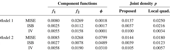
reported in Table1. Also included in the table are the values of MISE, ISB and IV ofφˆ. Although our primary concern is the estimation of the component functions, it is also of interest to see how good the produced two-dimensional density estima-torfˆ1(x)fˆ2(yφ(x))ˆ behaves. For this, we include in the table the values of MISE,
ISB and IV of the two-dimensional estimates computed using the optimal band-widths. For comparison, we also report the results for the two-dimensional local quadratic estimate defined at (3.1) that does not use the structure of the density. For this local quadratic estimator, we used its optimal bandwidth choice. The results confirm that our two-dimensional density estimator has much better performance than the local quadratic estimator, in both models.
One may be also interested in what happens if one ignores the presence of the nonconstantφ and estimatesfj withφˆ≡1, that is, estimates the simple product
model p(x, y)=f1(x)f2(y), (x, y)∈I. With the corresponding optimal
band-widths, the latter method produced (MISE,ISB,IV)=(0.0088,0.0026,0.0062)
for f1 and (0.0356,0.0168,0.0188) for f2 in the case of Model 1, and (0.0093,0.0031,0.0062) for f1 and(0.0320,0.0136,0.0184) for f2 in the case
of Model 2. Comparing these with the results in Table1, we see that estimatingφ
reduced significantly the values of MISE for the second componentf2, which
ap-pears to owe to the great reduction in ISB. Note that the accuracy of the estimation
TABLE1
Mean integrated squared errors(MISE),integrated squared biases(ISB)and integrated variance
(IV)of the estimators,based on500pseudo samples of sizen=400
Component functions Joint densityp
f1 f2 φ Proposed Local quad.
Model 1 MISE 0.0080 0.0269 0.0018 0.0137 0.0250 ISB 0.0025 0.0112 0.0017 0.0037 0.0216 IV 0.0055 0.0158 0.0001 0.0100 0.0034
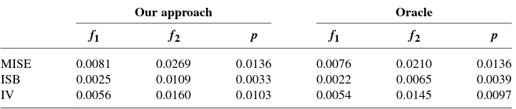
[image:19.486.56.413.506.616.2]TABLE2
Mean integrated squared errors(MISE),integrated squared biases(ISB)and integrated variance
(IV)of the estimators for Model3 (φ≡1),based on500pseudo samples of sizen=400
Our approach Oracle
f1 f2 p f1 f2 p
MISE 0.0081 0.0269 0.0136 0.0076 0.0210 0.0136 ISB 0.0025 0.0109 0.0033 0.0022 0.0065 0.0039 IV 0.0056 0.0160 0.0103 0.0054 0.0145 0.0097
of the second componentf2 relies on that ofφ, and that the method with φˆ ≡1
would produce a biased estimator off2.
Another thing that is of interest is that how our approach performs when there is no operational time, that is, the trueφ≡1. For this, we compared our approach that involves estimatingφ with the oracle estimators that make use of the knowl-edge thatφ≡1. The results are contained in Table2. In comparison with the oracle estimators, our approach produced slightly less accurate estimators of the compo-nent functions, but gave nearly the same MISE value for the estimator of the joint density function.
We also undertook a sensitivity analysis to check what happens if the struc-tural assumptions of the model are violated, that is, the density of (X, Y ) does not consist of three one-dimensional components but is simply a two-dimensional smooth density. For this we generated 500 samples of sizen=400 from a bivari-ate normal distribution with mean(1/2,1/2)and variance(1/3,1/3)with corre-lation 1/2, but truncated outside the parallelogram{(x, y): −(y/2)+(1/2)≤x≤
−(y/2)+1,0≤y≤1}. We compared the local linear and quadratic density esti-mators of the truncated normal density with the structured estimator that is based on the model (2.1). We found that, with the corresponding optimal bandwidths, the local linear estimator was slightly better than the local quadratic estimator, and it gave(MISE,ISB,IV)=(0.1015,0.0861,0.0154), while our structured estimation produced a better result,(MISE,ISB,IV)=(0.0729,0.0570,0.0159). This result suggests that the operational timeφintroduced into the multiplicative density adds a great deal of flexibility to the model so that it approximates quite well densities violating the independence assumption.
In practical implementation of our method, one may employ a K-fold cross-validation criterion to choose the bandwidths h andg. To be specific, one splits the whole dataset intoK (nearly) equal parts,{(Xi, Yi):i∈Jk},1≤k≤K. For
each partitionJk, one computes
CVk(h, g)=
Ipˆh,g,−k(x, y)
2dx dy− 2 |Jk|
i∈Jk
ˆ
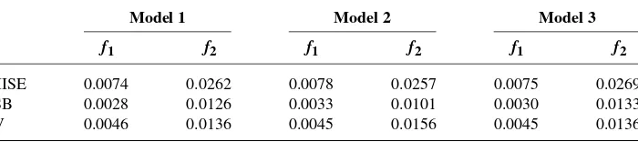
[image:20.486.73.435.115.192.2]TABLE3
Mean integrated squared errors(MISE),integrated squared biases(ISB)and integrated variance
(IV)of the estimators with tenfold cross-validated bandwidths,
based on500pseudo samples of sizen=400
Model 1 Model 2 Model 3
f1 f2 f1 f2 f1 f2
MISE 0.0074 0.0262 0.0078 0.0257 0.0075 0.0269 ISB 0.0028 0.0126 0.0033 0.0101 0.0030 0.0133 IV 0.0046 0.0136 0.0045 0.0156 0.0045 0.0136
where|Jk|is the size of the index setJk andpˆh,g,−k denotes our structured
den-sity estimate computed from the dataset with thekth partition being deleted, that is, from{(Xi, Yi):i /∈Jk}, based on the bandwidth choice(h, g). The above CV
criterion is common in density estimation; seePark and Marron(1990), for exam-ple. It is an estimate ofI(pˆh,g,−k(x, y)−p(x, y))2dx dy+(irrelevant term). The K-fold cross-validated choice is then defined by
(hcv, gcv)=(h,ˆ g)ˆ ×(1−1/K)1/5,
where (h,ˆ g)ˆ is the minimizer of CV(h, g)=Kk=1CVk(h, g)/K. Note that the
correction factor (1−1/K)1/5 is needed since (h,ˆ g)ˆ is suitable for the sample sizen(1−1/K)rather thann.
To see howK-fold cross-validated bandwidths perform in this particular prob-lem, we choseK =10 and applied the method to the three models. The results are summarized in Table3. Comparing the results with those in Tables 1and 2, we find that the cross-validated bandwidth selector works fairly well, giving com-parable performance with the MISE-optimal bandwidth. Motivated by this good performance, we used the tenfold cross-validated bandwidth in our data example in Section7.
7. Motor insurance data. As an example of implementing our method, we considered reported and outstanding claims from a motor insurance business line in Cyprus. For each claim, the dataset includes (EntryDate), (ClaimStatus) and (StatusDate). (EntryDate) is the date the claim was reported and entered the sys-tem, (StatusDate) is the date of the last update of (ClaimStatus) that has three categories: P for paid and settled; W for not paid but settled; O for open and not settled. Among 58,453 claims reported during the period January 12, 2004, to July 31, 2014, those claims with status O were deleted since for these claims the date of settlement was not observed. The number of deleted claims was 1865, and thus the number of the claims that we used to fit our model was 56,588.
[image:21.486.61.411.125.203.2]model (2.1) with I = {(x, y) :x ≥ 0, y ≥ 0, x +y ≤1}, we transformed the daily claim data in the following way. We first enumerated the calendar dates from 1 to 3854, with 1 corresponding to January 12, 2004, and 3854 to July 31, 2014, and then changed (EntryDate) and (StatusDate) to the respective inte-gers on the new discrete scale. This would result in a dataset for the variables
[(EntryDate), (StatusDate)−(EntryDate)]on the discrete triangular {(j, k):1≤
j≤3854,0≤k≤3853}. We then transformed them to(X, Y )by
X=(EntryDate)−1+U1
3854 , Y =
(StatusDate)−(EntryDate)+U2
3854 ,
where (U1, U2) is a two-dimensional uniform random variate on the unit square [0,1]2. Here, the perturbation by uniform random variates is done to make the con-verted data(X, Y )take values on the two-dimensional continuous time scale. This gives a converted dataset{(Xi, Yi):1≤i≤56,588}. We applied to this dataset
our method of estimating the structured densitypof(X, Y ).
We took a common bandwidthh=h1=h2for the estimation of the time
trans-formation φ, and a common bandwidth g=g1 =g2 for the estimation of the
component functions. We selected (h, g)by the tenfold cross-validated criterion described in Section6(K=10).
The results of the application of our method to the insurance claim data are shown in Figure3. In the left panel, the solid curve depicts the estimate of the time transformationφand the dashed (dotted) is a 90% (95%) pointwise bootstrap con-fidence band forφ. The 100(1−α)confidence bands[2φ(x)ˆ −Uα(x),2φ(x)ˆ − Lα(x)] were based on 1000 bootstrap samples, where Lα(x) andUα(x) are the
bootstrap estimates of the α/2 and(1−α/2) quantiles, respectively, of the dis-tribution of φ(x)ˆ . We note that the confidence bands are narrowed down to the
FIG. 3. The estimate of the time transformationφwith90%(dashed)and95%(dotted)pointwise confidence bands(left),the estimates of the first component functionf1 (middle)and the second
pointφ(x)ˆ =1 atx=0 because of our normalizationφ(ˆ 0)=1=φ(0), see (3.2). The bootstrap confidence bands indicate that the underlying transformation φ is not constant, so that the model (2.1) does not degenerate to the simple prod-uct modelp(x, y)=f1(x)f2(y)considered byMammen, Martínez Miranda and
Nielsen(2015). The estimatedφsuggests that the speed of time has an increasing tendency and that speed of time has increased by around 10% over the 10-year period considered. This is more or less in line with intuitive expectations to the model on how much improved technology has speeded up the process of getting incidents of claims settled. The decline ofφˆ after its peak might be because the company overall has decreased the number of employees when it saw the benefits of the advanced technology. The estimate of the first component measures busi-ness exposure, thus the middle panel of Figure 3indicates that the business line had increasing exposure in the first half of the period, but ran out later and perhaps was replaced by new products recorded in a separate dataset. The second compo-nent that measures time to settlement follows more or less the usual pattern known from motor insurance business lines that the claims development is quite fast.
One may use our estimated model to forecast the density on an unobserved area. In general, letSbe a subset of[0,1]2, outside of the observed areaI, where one wants to forecast the density. With the estimated density model p(x, y)ˆ = f1(x)fˆ2(yφ(x))ˆ , the relative mass of the probability onSwith respect to that onI
is estimated by
(7.1) A(S)=
S
ˆ
f1(x)fˆ2
yφ(x)ˆ dx dy.
The number of future observations that fall in the area S is then forecasted by
N (S)=n·A(S), where n is the sample size, that is, the total number of ob-servations inI. To apply the forecasting method to the motor insurance dataset and evaluate its accuracy, we re-estimated the model (2.1) now using the data ob-served until the year 2012. We forecasted the number of claims settled in the year 2013 according to the formula at (7.1). The actual number was 4547. Our ap-proach produced 4487, while the forecasting based on the simple product model
p(x, y)=f1(x)f2(y)gave 4226.
APPENDIX
A.1. Proof of Theorem2. In the following proof, we will use the symbolW
to denote functions that have bounded continuous partial derivatives, andW∗for continuous bounded functions. The symbols will be used for different functions, even in the same formula. They will denote univariate functions and bivariate func-tions as well. Furthermore, for simplicity of notation, we assume thath1=h2=h.
Put(x)=logφ(x)ˆ −logφ(h)ˆ − [logφ(x)−logφ(h)]. We will show that
(A.1) (x)=Op
It can be shown by slightly modified and simpler arguments that
(A.2) logφ(h)ˆ −logφ(h)=Op
n−2/5.
The bounds (A.1) and (A.2) imply (3.5). For a proof of (3.6), one may show, in-stead of (A.1) and (A.2), the slightly stronger claim
(A.3) sup
x∈[0,1−]
E2(x)=On−4/5.
This can be done by a slightly more careful use of the arguments in the proof of (A.1). For a proof of (3.7), one makes use of exponential inequalities for the terms of the stochastic expansion that we will consider below in the proof of (A.1).
We now come to the proof of (A.1). By Taylor’s expansion, one gets that
(x)=
x
h
Gˆ
11(u)− ˆG10(u)Gˆ01(u) ˆ
G02(u)− ˆG01(u)2
−G11(u)−G10(u)G01(u)
G02(u)−G01(u)2
du
=1(x)+2(x)+3(x)+R(x),
(A.4)
where1comprises all linear terms of the form
x
h W (u)(Gˆj k(u)−Gj k(u)) duof
a Taylor expansion of the integrand of the integral in (A.4). The second term2
collects those terms of quadratic order, hxW (u)(Gˆj k(u)−Gj k(u))(Gˆjk(u)− Gjk(u)) du, and 3 contains all cubic terms. Among these linear, quadratic and
cubic terms, the most complex terms are those that involve Gˆ11. Note that Gˆ11
contains a product of two partial derivatives, whereas Gˆj k for (j, k)=(1,1)
in-cludes at most one partial derivative. For the remainder term R, it holds that
R(x)=Op(n−2/5). This bound follows from
EGˆj k(u)−Gj k(u)
4=
On−2/5
and a bound on the variance ofhx(Gˆj k(u)−Gj k(u))4du. One can show that the
bound onRholds uniformly for 0≤x≤1−. We now prove
(A.5)
x
h
W (u)Gˆ11(u)−G11(u)
du=Op
n−2/5.
Using the same arguments as for the proof of (A.5), one can show that the other terms of1are of orderOp(n−2/5). This implies that
(A.6) 1(x)=Op
n−2/5.
For the proof of (A.5), we redefine the vectora(u, v;x, y)in Section3as
au, v;u, v=1,u−u2/ h2,v−v2/ h2,