This is a repository copy of Robust control strategies for multi-inventory systems with
average flow constraints..
White Rose Research Online URL for this paper:
http://eprints.whiterose.ac.uk/89773/
Version: Accepted Version
Article:
Bauso, D., Blanchini, F. and Pesenti, R. (2006) Robust control strategies for
multi-inventory systems with average flow constraints. Automatica, 42 (8). 1255 - 1266.
https://doi.org/10.1016/j.automatica.2005.12.006
Reuse
Unless indicated otherwise, fulltext items are protected by copyright with all rights reserved. The copyright exception in section 29 of the Copyright, Designs and Patents Act 1988 allows the making of a single copy solely for the purpose of non-commercial research or private study within the limits of fair dealing. The publisher or other rights-holder may allow further reproduction and re-use of this version - refer to the White Rose Research Online record for this item. Where records identify the publisher as the copyright holder, users can verify any specific terms of use on the publisher’s website.
Takedown
If you consider content in White Rose Research Online to be in breach of UK law, please notify us by
Robust control strategies for multi–inventory systems with
average flow constraints
Dario Bauso
a, Franco Blanchini
b, Raffaele Pesenti
aa
Dipartimento di Ingegneria Informatica, Universit`a di Palermo, Viale delle Scienze, I-90128 Palermo, ITALY
b
Dipartimento di Matematica ed Informatica, Universit`a degli Studi di Udine, Via delle Scienze 206, 33100 Udine, ITALY
Abstract
In this paper we consider multi–inventory systems in presence of uncertain demand. We assume that i) demand is unknown but bounded in an assigned compact set and ii) the control inputs (controlled flows) are subject to assigned constraints. Given a long–term average demand, we select a nominal flow that feeds such a demand. In this context, we are interested in a control strategy that meets at each time all possible current demands and achieves the nominal flow in the average. We provide necessary and sufficient conditions for such a strategy to exist and we characterize the set of achievable flows. Such conditions are based on linear programming and thus they are constructive. In the special case of a static flow (i.e. a system with 0–capacity buffers) we show that the strategy must be affine. The dynamic problem can be solved by a linear-saturated control strategy (inspired by the previous one). We provide numerical analysis and illustrating examples.
Key words: Inventory control, Robust control, Bounded disturbances, Manufacturing systems, Linear programming.
1 Introduction
Multi–inventory systems [12,26] are formed by buffers, where raw materials/subassemblies/finished products are stored, connected by processing links, along which items are produced or transported. Such systems are met in several different contexts, such as manufacturing [2,7,8,14,16,20,21], network routing [13], communica-tions [9], water distribution [15], logistics and traffic control [18]. Hence, their control is of relevant economic interest. The control concerns storage and processing operations and aims at meeting the external demand of finished products [10,12].
In the literature, there are many contributions on the design, and possibly the optimization, of the system con-trols with respect to static criteria in the assumption that the demand is known in advance (see, e.g., [24]). Unfortunately, many real systems work in uncertain and time–varying conditions. Thus, a feedback approach is
⋆
This paper was not presented at any IFAC meeting. Cor-responding author F. Blanchini. Tel. +39 0432 558466. Fax +39 0432 558499.
Email addresses: [email protected](Dario Bauso),
[email protected](Franco Blanchini),
[email protected](Raffaele Pesenti).
preferable [1,13,14,19] to assure robustness against un-certain events such as failures or unknown demand rate. In this context, several authors deal with the problem of transient optimality (see, e.g., [2,17,19,22]) and near-optimality (see, e.g., [25]). However, few of them explic-itly consider uncertainties in the demand or supply flows (see, e.g., [4,6,7]).
We pursue a deterministic approach by assuming that the external input (we will name it for brevity “the demand”) is unknown–but–bounded within given con-straint sets. Under this assumption, the basic problem we are investigating is the stability of the multi-retailer system. In a context of fluid models, the stability of the system consists in keeping the buffer levels within as-signed constraints or driving them to prescribed levels [4] [6]. In those references it is shown that for continuous– time models there exists a strategy assuring convergence to any target buffer level if a certain “control dominance” necessary and sufficient condition is satisfied. Some op-timality criteria for the transient are considered in [3].
ma-trix is a “large one”). Therefore we have a degree of free-dom in choosing, at each time, the workload distribution among controlled links that satisfies at each time the current demands. Beside satisfying at each time the cur-rent demand, we are also concerned with the long–term utilization of the system. At a certain time, a generic link may be requested to work harder, than expected in the average, or to be underutilized due to demand fluc-tuations. However, the average utilization of the links should be adapted to the “average” behavior of the de-mand and possibly determined by a (steady–state) op-timality criterion. This problem is important because in many context, balancing between links is fundamental since over–utilization of some links may cause failures or produce high costs.
In this work we simultaneously consider the two follow-ing aspects.
• Instantaneous fluctuations— These are assumed un-known due to the large number of unpredictable fac-tors that influence the demand. The control must face all possible variations, within prescribed limits, in or-der to meet the demand. So, these fluctuations can require a control flow which is, instantaneously, com-pletely unbalanced with respect to the nominal one. • Long term information— Forecasts about long–term
average demand values are generally much more re-liable. Quite accurate statistics over long–time hori-zons are often available. Besides, long–term values are sometimes fixed (for instance established by contract). The long–term average demand, henceforth also called nominal demand, should be faced, in the average, by the nominal flow, whenever possible.
Therefore we are seeking for a stabilizing strategy capa-ble of balancing the flow in the long run. A basic ques-tion is the following. Given the system structure and the controlled flows constraints and assumed that the de-mand has a known (deterministic) average value, can we find a stabilizing strategy which assures, in the average a prescribed controlled value? As we will see by means of a trivial examples such a strategy does not exists even if the nominal flow is feasible and feeds the nominal de-mand in steady–state. It will be apparent that this fact is due to the simultaneous presence of flow constraints and demand uncertainties.
We will refer to controlled process matrix that, in gen-eral, may not be the incidence matrix of graph. In this sense, a main contribution of the paper is in the gener-ality of the topology of the systems, which are not nec-essary networks. The main results of the paper are re-ported next.
• We first consider static strategies (i.e. we assume 0– capacity buffers). We provide necessary and sufficient conditions for the existence of a strategy which is able
to meet all the possible demands and assures the de-sired flow average, whenever the demand meets its nominal average. Such conditions are based on linear programming and are constructive.
• We characterize the set of all flows corresponding to the nominal demand which can be achieved in the average.
• We show that, if the necessary and sufficient condi-tions are satisfied, then the static strategy is affine. Such an affine function characterizes the actual age flows even in the cases in which the demand aver-age is different from the nominal one.
• We show that the very conditions, valid in the static case, are sufficient for the existence of a dynamic strat-egy, based on the feedback of the buffer levels. These conditions are also necessary under appropriate, quite general, assumptions.
• We show that the proposed feedback strategy is a linear-saturated dynamic control. The introduced dy-namics is, basically, an integrator that gets rid of the load unbalancing. The control synthesis is based on the mentioned linear programming conditions. • We prove that the problem of establishing whether a
nominal flow is achievable or not is an easy problem. Actually, this is done through a polynomial algorithm that selects a candidate strategy and verifies the men-tioned conditions at each iteration.
The paper will finally present applications and discus-sion of the proposed theory.
2 Problem Formulation
Consider the following continuous time system
˙
x(t) =Bu(t)−w(t), (1)
wherex(t)∈IRn is a vector whose components are the buffer levels, u(t) ∈ IRm is the controlled flow vector,
B is the controlled process matrix and w(t) ∈ IRn is an exogenous (uncontrolled) input, typically modeling demand, whose value is externally determined. To model backlogx(t) may be less than zero.
We assume that uand w are subject to the next con-straints
u(t)∈ U ={u:u−
≤u≤u+}, (2)
whereu−andu+are assigned vectors and the expression is to be intended component-wise. We assume thatwis constrained as follows
w(t)∈ W, (3)
Assumption 1 MatrixBhas full row rank.
If the above assumption is not satisfied, the system is unreachable. As we will see soon, the problem becomes trivial ifB is square therefore we will consider the case in whichBis a “fat matrix”.
Given a vector function of timef : IR+→IRn we
intro-duce the following notation
Av[f] = lim
T→∞
1 T
T
Z
0
f(t)dt. (4)
FunctionAv[f] will be referred to as the deterministic average off, henceforth theaverage, and we will always assume that such a value exists whenever considered.
Assumption 2 The setW includes w¯ = Av[w] in its relative interior1.
We will consider static and dynamic stabilizing policies for the system according to the following definitions.
Definition 3 The functionΦ : IRn → IRm is a static balancing strategyif foru(t) = Φ(w(t)),
Bu(t) =w(t),
andu(t)∈ U, for allw(t)∈ W, for allt≥0.
If a static balancing strategy is applied, as a consequence we have ˙x(t) = 0. Therefore (from a ideal point of view) the buffer level remains bounded since the system meets at each time the current demand. Clearly this is not a feedback strategy and the resulting system is not stabi-lized2.
Our ultimate goal is solving the dynamic problem of steering the system buffer to the neighborhood of a pre-scribed level.
Definition 4 Givenǫ >0and a reference valuex, an¯ ǫ -stabilizing strategyis a feedback control for which there exists a continuous positive functionφ(t), monotonically decreasing and converging to0ast→ ∞such that for all w(t)∈ Wand for allx(0), the conditionsu(t)∈ U and
kx(t)−x¯k ≤max{kx(0)kφ(t), ǫ}
hold true.
1
we mean that ¯wis an interior point ofWwith respect to
the smallest linear subspace including it, for instance given a vectorv6= 0, 0 is in the relative interior of a segment joining vand−v
2
indeed infinitesimal perturbations onwmay cause buffer
overflow
We introduce the following basic conditions [4] as a pre-liminary result.
Theorem 5 For the considered system
i there exists a static balancing strategy as in Definition 3
if and only if
W ⊆BU; (5)
ii there exists a feedback stabilizing strategy as in
Defi-nition 4 if and only if
W ⊆int{BU}. (6)
Henceforth, we assume that the appropriate necessary and sufficient condition is met (depending on which kind of strategy we are considering). Assume to apply either a balancing or anǫ-stabilizing strategy. As a consequence, x(t) remains constant or bounded. Then, by integrating (1) we have that, necessarily,
lim
T→∞
1 T
T
Z
0
[Bu(t)−w(t)]dt= lim
T→∞
1
T [x(t)−x(0)] = 0,
which implies that the average value ofwis equal to the average value ofBu
B Av[u(t)] =Av[w(t)]. (7)
Given a nominal average flow ¯w, unlessB is square (the problem would be trivial in this case) there are several possible vectors (average controlled flows) ¯u=Av[u(t)] such that B¯u= ¯w. By exploiting this redundancy, we are actually interested in selecting a nominal flow ¯uthat supports the average of the demand Av[w] whenever Av[w] = ¯w∈ W.
Formally, the problem is the following.
Problem 6 Assume that the average w¯ ∈ W is given. Consider the feasible flowu¯∈ U such that
Bu¯= ¯w.
Provide a yes–no answer to the question: does there ex-ist a static balancing (or dynamicǫ–stabilizing) strategy such that wheneverAv[w] = ¯w thenAv[u] = ¯u? In the case of a positive answer we will say thatu¯is achievable.
We stress that, given ¯w∈ W, not all the vectors ˆusuch thatBuˆ= ¯wcan be achieved as average flows, as shown next.
Example 7 Consider the scalar system
˙
u
2
1
u
u
au
bA
B
D
F
E
C
[image:5.612.48.277.33.177.2]H
G
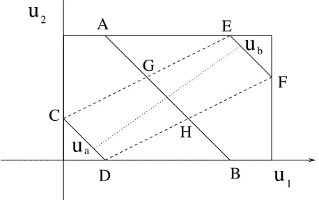
Fig. 1. The achievable averages where
0≤u1≤5, 0≤u2≤3, 1≤w≤7.
Assume thatAv[w] = 4. The all candidate average flows are those such that
¯
u1+ ¯u2−4 = 0,
precisely those on the central lineA–B in Fig. 7. Now the feasible flows to meet the demandu1+u2 =w= 1 are those on the line C–D, while the feasible flows to meet the demand u1+u2 = w = 7 are those on the lineE–F. Now, if the demand periodically jumps from1 to7 as follows:w(t) = 1 for kT ≤ t < kT +T /2 and w(t) = 7forkT +T /2≤t <(k+ 1)T then its average isw¯ = 4but it can be faced only by points of the type ua andub respectively. It is therefore clear that the only
suitable average values are those on the lineA–B which are included between the two dashed lines (segmentG– H). Actually it is not difficult to see that, for a generic
¯
wthe achievable average flowsu¯for this problem are all the points on the lineu¯1+ ¯u2= ¯wconfined between such dashed lines (i.e. such that−1≤2¯u2−u¯1≤1).
In the following sections we will solve constructively the problem for both static and dynamic strategies.
3 Achievable average: the static case
In this section we consider the case in which the con-trolled flow is a function of the demand w so that Bu(t) = w(t). Note that this control strategy can not stabilize the queue lengths since the time derivative of the queue lengths is made zero. This situation occurs in several problems (for instance in power supply). This section has to be considered as a prelude to the dynamic case in which we will use the necessary and sufficient conditions derived here.
For the simple notations we work under the following assumption.
Assumption 8 The nominal average “demand” is zero, i.e.w¯=Av[w] = 0∈ W.
This is not a restriction because under the conditions (5) or (6) there existsu0(we will assume equal to ¯ufor convenience) such thatBu0 = ¯w, the nominal average. Then we can translate the problem by writing the new model
˙
x(t) =B(u(t)−u0)−[w(t)−w¯] =Bδu(t)−δw(t)
and by translating the constraints as
u−
−u0≤δu(t)≤u+−u0, δw(t)∈ W −w.¯
where Av[δw] = 0. If we assume u0 = ¯uthe question is weather a static balancing strategy exists such that any null average demand implies a null average flow. The following theorem, whose proof will be given later, provides an answer.
Theorem 9 Under Assumption 1 and 2 let condition (5) be satisfied. Then there exists a static balancing strategy that achieves the averageAv[u] = 0wheneverAv[w] = 0 if and only if there exists a “tall” matrixD m×nsuch that
BD=I (8)
u−
≤Dw(i)≤u+, i= 1, . . . , s. (9)
wherew(i)are the vertices ofW. Moreover, if such nec-essary and sufficient conditions are satisfied, then the static strategy is linear
u(t) =Dw(t). (10)
The previous theorem allows us to check a single candi-date ¯uwe fixed to zero. We can now characterize theset of achievable average flows, namely the set of all vectors such thatAv[w] = 0 impliesAv[u] = ¯u∈ U.
Corollary 10 The set of all achievable average flows, provided that a suitable static balancing strategy is ap-plied, is made up by all the vectorsu¯∈ker[B]such that there exists a matrixD,m×n, with
BD=I (11)
u−≤Dw(i)+ ¯u≤u+, i= 1, . . . , s. (12)
In this case the static strategy is affine
u=Dw+ ¯u.
We have seen that as long as a strategy achieving the average exists, this has to be linear (or affine taking into account possible translations onw). As a consequence of the linearity we have the following property.
Corollary 11 If the necessary and sufficient condi-tions (8) and (9) are satisfied, then the average con-straints are satisfied not only on the infinite horizon, but on every finite horizon as well, in the sense that for all T >0
1 T
T
Z
0
w(t)dt= 0 implies 1 T
T
Z
0
u(t)dt= 0.
Remark 12 It should be noticed that, if the demand av-erage is not the nominal one, butAv[w] = ˆw, then the corresponding average flow is characterized by
Av[u] =DAv[w].
This means thatDmay be thought of as a “partitioning law” for the workload Av[u] and thus chosen via some optimality criterion.
3.1 Proof of the theorem
To prove the theorem we need the next lemma.
Lemma 13 Consider a convex cone C ⊂ IRn centered in0with a non–empty interior. Consider two subspaces YandZ ⊂IRn and define
ˆ
Y =. Y\C, Zˆ=. Z\C.
Assume that Yˆ includes an element interior to C, y ∈ int{C}. ThenY ⊆ˆ ZˆimpliesY ⊆ Z.
PROOF. We initially observe that, since Y and Z are subspaces, we can prove the lemma by showing that dim(YTZ) = dim(Y). To this end, note that, as C is not empty, dim(C) = n; as C and Y are poly-topes,y ∈ int{C}implies that there exists δ >0 such that y+δe(i) ∈ Yˆ, for each vector e(i) belonging to a basis of the subspaceY. Hence, dim( ˆY) = dim(Y). Finally, as YTZ ⊇ YTZTC, then ˆY ⊆ Zˆ im-plies YTZ ⊇ Yˆ. Hence, dim(YTZ) ≥ dim(Y). As dim(YTZ) ≤ min{dim(Y), dim(Z)} we obtain dim(YTZ) =dim(Y). 2
We can now prove the theorem.
Sufficiency. We assume that (8) and (9) hold and prove that (10) is the desired strategy. Indeed, strategy (10) is static and balancing, sinceu(t) =Dw(t) implies
Bu(t) =BDw(t) =w(t). In addition, for allw∈ W, we have thatw=Pαiw(i),Pαi= 1,αi≥0, then
u=Dw=XαiDw(i)∈ U.
Strategy (10) also achieves the averageAv[u] = 0 when-everAv[w] = 0, sinceu(t) =Dw(t) implies alsoAv[u] = Av[Dw] =DAv[w].
Necessity. We assume that there exists a static balanc-ing strategyu= Φ(w) such thatu∈ U for allw ∈ W and such thatAv[w] = 0 impliesAv[u] = 0 and we prove that (8) and (9) hold. Given the nonnegative unit–sum vector α = [α1 α2. . . αs], α ≥ 0, ¯1Tα = 1 consider a
periodic demandw(t) of periodT defined as follows
w(t) =w(k),
kX−1
i=0
αiT ≤t≤ k
X
i=0 αiT,
fork = 1,2, . . . , s, withα0 = 0 Namely,w(t) assumes the vertex valuew(i)for the portion of periodα
iT. This
demand is feasible and its average is
Av[w] =
s
X
i=1
αi w(i).
Now, no matter how theαiare chosen, the above static
balancing strategy feeds any possible demand w(i) through a controlled flowu(i)= Φ(w(i)) which verifies
BΦ(w(i)) =w(i).
As a consequence the average flow is
Av[u] =
s
X
i=1
αi Φ(w(i)) = s
X
i=1
αiu(i).
Denote byW = [w(1)w(2) . . . w(s)] the matrix including the vertices of W and by U = [u(1) u(2) . . . u(s)] the corresponding input values (note that this meansBU = W). In view of the assumption, we have thatAv[w] = 0 impliesAv[u] = 0, which can be written as
W α= 0, ⇒ U α= 0, (13)
(actuallyW α = 0 iff U α = 0). Therefore the positive kernel of W, precisely the intersection of ker[W] with the positive hortant, is included in the positive kernel of U.
We remind now that 0 belongs to the relative interior of Wby Assumption 2.
Then in theαspace, there exists a positive vector ˆα >0, ¯
lemma and claim that
ker[W]⊆ker[U].
On the other hand we have, by construction thatW = BU and thenU α= 0 impliesW α=BU α= 0, so that ker[U] =ker[W].
This means that the columns ofU can be generated as linear combination of the columns ofW and vice-versa and therefore the two matrices have the same row rank. Therefore, there exists a matrix ˆD m×nsuch that
U = ˆDW.
Then
W =BU =BDW.ˆ
Now, ifW has full row rank, this impliesBDˆ =I and then (8). Actually, the equation implies thatBDˆ, is the identity within the subspace generated by the column of W. We show now that we can always find a right inverse ofB, precisely a matrixD such thatBDˆ =I. Assume thatWhas not full row rank and take the matrix Q=P−1such that
QW =
" ˜
W1
0
#
and let hD˜1 D˜2
i .
= ˆD P
with ˜W1 full row rank equal toρ. Consider the equa-tionBDWˆ =W and premultiply both its sides byQas QBDWˆ =QBDP QWˆ =QW we achieve by substitu-tion
QB hD˜1 D˜2
i "W˜1
0 # = " ˜ W1 0 # ,
where ˜D1has necessarily full column rank (equal toρ). Note that we can replace ˜D2 by a tall matrix ∆ (with n−ρcolumns)
QB hD˜1 ∆
i "W˜1
0 # = " ˜ W1 0 #
Take ∆ such thatQB∆ =h0 I
iT
(this is possible be-causeQB has full row rank) and augment the previous equation as follows
QB hD˜1 ∆i
" ˜
W1 0
0 I
#
=
" ˜
W1 0
0 I
#
.
Note that the rightmost matrix has full row rank. By multiplying on the left byP we achieve
B hD˜1 ∆iQ
| {z. }
=D
P
"
˜ W1 0
0 I
#
| . {z }
=[W W∗]
=BD[W W∗
] =
=P
" ˜
W1 0 0 I
#
= [W W∗
]
with [W W∗
] of full row rank. As previously observed, this means that BD = I. Now we have to show that U =DW. This is easy
DW =hD˜1 ∆
i Q P " ˜ W1 0 #
=hD˜1 ∆
i "W˜1
0
#
=
=hD˜1 D˜2
i "W˜1
0
#
=hD˜1 D˜2
i Q P " ˜ W1 0 #
= ˆDW =U.
Then, for each roww(k)ofW Dw(k) =u(k) = Φ(w(k)) and thus (9) is automatically satisfied. 2
Example 14 (Example 7 cont’d) Let us briefly consider again the simple system of Example 7. Since the long– term average demand is w¯ = 4we can select a nominal flowu¯= [2.5 1.5]′. By translating the axes to the origin u0= ¯u, we have the new model
˙
x(t) = (u1(t)−2.5) + (u2(t)−1.5)−(w(t)−4) =δu1(t) +δu2(t)−δw(t),
where−2.5 ≤ δu1(t) ≤ 2.5, −1.5 ≤ δu2(t) ≤ 1.5, and −3≤δw(t)≤+3.Now, there exist a variety of matri-cesDthat verify conditions (8) and (9). As an example, we can chooseD=23 13′. The resulting static strategy for the translated problem is then
δu(t) =
"
2/3
1/3
#
δw(t),
which in the original axes takes on the form
u(t) =Dδw+u0=
"
2/3
1/3
#
δw(t) +
"
2.5
1.5
#
.
There are counterexamples which prove that Theorem 9 does not hold when 0 6∈ rel int{W}, (in general when
¯
4 Achievable average flows with dynamic strategies
Here we show how to achieve an average flow by a dy-namic stabilizing strategy. The main results of the sec-tion is Theorem 19, which basically states that the con-ditions for the existence of a dynamic strategy which, achieves a certain average are the same of the static case. We will first show, in the next subsection, that condi-tions (8) and (9) are sufficient for the existence of a dy-namicǫ–stabilizing strategy of the form
˙
y(t) =f(y(t), x(t), w(t))
u(t) = g(y(t), x(t), w(t)). (14)
To provide results about necessity of (8) and (9) we need to better characterize the class of dynamic strategies by additional assumptions. This will be done in the subse-quent subsection.
4.1 Sufficiency of the conditions
Let assumptions (8) and (9) be satisfied and consider the corresponding matrixD. Equation (8) means thatDis a right inverse ofBand it is a standard property of linear algebra that this is equivalent to the existence of two matricesC andF which “square”B and D producing two matrices inverse to each other, namely such that
"
B C
# h
D Fi=I. (15)
Consider the following augmented system
˙
x(t) = Bu(t)−w(t)
˙
y(t) =Cu(t). (16)
The additional dynamic variable ˙y(t) = Cu(t) has the goal of keeping trace of the load unbalancing with respect to the desired average 0.
The first step is to show that under (8) and (9), the ex-tended system (16) satisfies the stabilizability conditions (6) as well (in the extended state–space), precisely for allw∈ W there existsu∈ U such that
"
w
0
#
=
"
B
C
#
u,
or equivalently that, for allw∈ W, there existsu∈ U such that
u=hD F
i "w
0
#
=Dw.
The existence of suchuis an immediate consequence of (9). Indeed, it is easy to verify that, if W ∈ int{BU}, then theuwhich corresponds towis in the interior of the extended set. Then the problem can be solved as follows.
• DetermineD such that (8) and (9) are satisfied. • DetermineC andF such that (15) is satisfied. • Design a control which stabilizes (16).
Observe that Theorem 5 applied to the extended sys-tem (16) guarantees the existence of such a stabilizing control.
Here we propose a new strategy based on a variable transformation. In the following we exploit (for the first time) the structure of the setU. Consider the new vari-ablez(t) defined as
z(t) =hD Fi
"
x(t) y(t)
#
,
"
x(t) y(t)
#
=
"
B C
#
z(t)
This variable satisfies the equation
˙
z(t) =u(t)−Dw(t). (17)
The new system (17) is decoupled in its state variable, precisely it is equivalent to
˙
zi(t) =ui(t)−Diw(t), (18)
where we have denoted byDitheith row ofDand where
u−
i ≤ui≤u+i. Denote by
ρ−
i = min w∈W Diw, ρ+i = maxw∈W Diw,
The stabilizability conditions are equivalent to the fact that for allw∈ W
u−
i < ρ
−
i < ρ
+
i < u
+
i.
Henceforth, without restriction, we consider the single– buffer case, namely the scalar system
˙
z(t) =u(t)−r(t),
with
ρ−
≤r(t)≤ρ+, u−
≤u(t)≤u+.
Define the saturated control (see Fig. 2)
withκ >0 and where
sat[α,β](ζ) =
β, if ζ > β, ζ, if α≤ζ≤β,
α, if ζ < α.
We will use the same notation (19) for the multi–input control derived applying the formula component–by– component. Note that this control function is Lipschitz
+
u
u
u /
+κ
κ
u /
u
[image:9.612.78.246.148.277.2]z
Fig. 2. The function (19)
continuous. For κ→ ∞, the control (19) converges to the bang bang control
bb[u−,u+](ζ) =
u+, if ζ >0,
0, if ζ= 0,
u−
, if ζ <0,
which is of the type considered in [4].
Theorem 15 The variable z(t) with the control (19) converges to the interval [−u+/κ,−u−
/κ] (which in-cludes0 as an interior point). Therefore the global sys-tem converges to the corresponding hyper–box (i.e. that delimited by−u+
i /κ≤zi≤ −u−i /κ,i= 1,2, . . . , m).
PROOF. The proof derives from the fact that, forz ≥ −u−
/κ, we have that the control is saturated to its lower levelu=u−, then
˙ z=u−
−r≤u−
−ρ−
<0. (20)
Conversely forz≤ −u+/κwe have thatu=u+, then
˙
z=u+−r≥u+−ρ+>0. (21)
Thereforez(t) reaches the interval in finite time and is ultimately confined in it. 2
As a consequence of the previous theorem we have that, choosingκlarge enough, we can boundzin an arbitrar-ily small interval. Therefore we achieveǫ–stability. We
have now to show that the controller so obtained sat-isfies the average requirement. Indeed variable z(t) re-mains bounded sokz(t)−z(0)k ≤ξ.By integrating (17) we have that
1 T
T
Z
0
u(t)dt− 1 T
T
Z
0
Dw(t)dt= z(T)−z(0)
T →0
asT → ∞. This yields
Av[u] =Av[Dw],
that is all we need to claim that sufficiency of (8) and (9) is proved.
We briefly consider now the case in which the control is allowed to be discontinuous. This case is important in all the systems in which several controlled arcs are of the switching (on–off) type.
Corollary 16 The system equipped with the bang–bang controlu=bb[u−,u+](z)is such thatz(t)→0. The origin is reached in finite time which is equal to
τmax= max i max{
zi(0)
−u−
i −ρ
−
i
, −zi(0) u+i +ρ
+
i
}.
PROOF. It is an easy consequence of the fact that the derivative can be bounded forz >0 as in (20) and for z <0 as in(21). 2
Remark 17 The proposed strategy works under mea-surement errors. Bounded meamea-surement errors on x(t) imply bounded errors onz(t). By reasoning component-wise we achieve systems of the form
˙
z=sat[u−,u+](−κ(z+δz))−r
whose state remains bounded as long as the errorδz is
such. Precisely via elementary analysis it can be shown that if|δz| ≤δmeas thenzwill be ultimately confined in
the interval[−(ǫ+δmeas),(ǫ+δmeas)].
4.2 Proof of necessity
In this section we show the necessity of conditions (8) and (9) for the existence ofǫ–stabilizing strategy in the general class that satisfy the next assumption.
Assumption 18 The strategy must assure
• Uniqueness at steady state: For each vertexw(k)ofW there exists a correspondingu(k) such that forw(t)≡ w(k)and for all initial condition int
0as above
1 τ
tZ0+τ
t0
(u(σ)−u(k))dσ
≤ψ(τ),
whereψ(τ)is a positive monotonically decreasing con-tinuous function converging to0 asτ→ ∞.
The assumption means that i) the additional dynam-ics represented by variabley(t) must be bounded under bounded disturbancesw“at least after some time”; and that ii) for a constantw(k) the strategy replies with a unique vectoru(k) in the average. In the case of a con-tinuous control this just means that, at steady state, w(k)is faced by a precise flow vectoru(k). The strange formulation is due to the fact that for some discontinu-ous strategies the valueu(k)may be a value not actually achieved at any time. For instance consider the system
˙
x=u−w
with the controlu=−bb[−1,1](x). Ifwis constant equal to 1/2, then the correspondingu= 1/2, but the value is never achieved.
We show now that under Assumptions 1 and 2, if there exists anǫ–stabilizing strategy which satisfies also As-sumption 18 and which meets the average valueAv[u] = 0 wheneverAv[w] = 0 for allw(t)∈ W, then (8) and (9) must be satisfied.
Consider the matrixWmade up by the vertices ofWand fix a positive vectorαsuch thatW α= 0 andPsi=1 αi =
1 (the fact thatαcan be positive is due to Assumption 2). GivenT >0 consider again the demandw(t) periodic of periodT, defined as follows
w(t) =w(k), T
k≤t≤Tk+1 where Tk= k−1
X
i=0 αiT,
whereα0 = 0, having averageAv[w] =W α. Let ¯x= 0 and kx(t0)k ≤ ν and ky(t0)k ≤ µ for t0 = 0. For T large enough these bounds are true, by assumption, for any t0 chosen as any“switching time” of w (just take T αi ≥¯tfor alli). Assume that forAv[w] = 0Av[u] =
0. Then the control average on [0, T] is (noticing that [Ti+1−Ti]/T =αi) is the limit of the following function
h(T)=. 1 T
T
Z
0
u(t)dt= 1 T
s
X
k=1
TZk+1
Tk
u(t)dt=
= 1 T
s
X
k=1
αku(k)+
1 T
s
X
k=1
TZk+1
Tk
u(t)dt−
s
X
k=1
Tk+1−Tk
T u
(k)=
= 1 T
s
X
k=1
αku(k)+
1 T
s
X
k=1
TZk+1
Tk
h
u(t)−u(k)idt=
= 1 T
s
X
k=1
αku(k)+ s
X
k=1 αk
1 Tk+1−Tk
TZk+1
Tk
h
u(t)−u(k)idt
| {z }
→0,asT→∞
.
The fact that the rightmost quantity converges to 0 as T → ∞, follows from Assumption 18. Since alsoh(T)→ 0, we have that
1 T
s
X
i=1
αiu(k)= 0.
Since α > 0, we have proved condition (13). The re-maining part of the proof proceeds exactly as the proof of Theorem 9 so necessity is proved.
We can then formalize the result as follows.
Theorem 19 Under Assumptions 1 and 2, let the sta-bilizability condition (6) be satisfied. Then there exists a control, in the class of strategies satisfying Assump-tion 18, which achieves the average0wheneverAv[w] = 0 if and only if there exists a “tall” matrixD m×nsuch that (8) and (9) are satisfied.
Remark 20 The provided theory can be easily applied to systems with production/transportation delays along the lines proposed in [5] for discrete–time systems. The extension to the continuous–time case is simple as we show next. Consider the model
˙
x(t) =B0u(t) +
s
X
k=0
Bku(t−τk)−w(t)
whereτk are known delay (see [5] for details). Consider
the variable “inventory position”
xip(t) =x(t) + s
X
k=1
t
Z
t−τk
Bk u(σ)dσ
By differentiatingxip we derive the following equation
˙
xip(t) =Bu(t)−w(t)
where we have defined B =. Psk=0Bk. Since u(t) is
Then the exposed theory applies without modifications if we deal with the problem of keepingxip(t)bounded.
Note that this strategy provides boundedness, but not epsilon-stabilization (except when ε is larger than
P
kτkmaxu∈U||Bku||). Achieving regulation would
re-quire controller design which takes into account delays. This is a challenging problem, especially when the delays are unknown and/or time-varying (which is usually the case in practice). An attempt to solve this problem in the case of communication networks has been made by [23].
5 Existence of achievable average flows
In this section, we show that verifying whether a given average flow is achievable is an easy problem. This can be accomplished in polynomial time by an algorithm that iteratively selects a candidate control strategy and checks if the necessary and sufficient conditions are isfied. The algorithm stops when the conditions are sat-isfied returning a possible strategy, or establishes that no strategy exists such that the average flow ¯uis achievable. To study the difficulty of such a problem, henceforth we assume thatWis known through its external represen-tation, i.e., it is described by means of the inequalities defining its facets.
We initially determine whether a given flow ¯u ∈ U is achievable. More formally we face the following prob-lems.
Problem 21 Assume that a feasible flowu¯∈ U ∩ker[B], and a matrixD∈IRm×n, such thatBD=I, are given. Provide a yes–no answer to the question whether u¯ is achievable with the strategyu=Dw+ ¯u.
Problem 22 Assume that a feasible flowu¯∈ U ∩ker[B] is given. Provide a yes–no answer to the question whether there exists a matrixD∈IRm×nsuch thatu¯is achievable with the strategyu=Dw+ ¯u.
Observe that, in general, an achievable flow may not ex-ist. This fact is due to thesimultaneous presence of con-trol constraints and input uncertainty. Indeed it is triv-ial to see that, when the demand setW is a singleton, any flowu∈ U such thatBu=wis achievable. On the other hand, if the control is unbounded, i.e.,u+= +∞ and u−
= −∞, conditions (11) and (12) in Corollary 10 hold trivially. Therefore the following questions are natural: given W, which is the “smallest” box U for which an achievable value exists? Or, givenU, which is the “largest” uncertainty setWfor which an achievable value exists? These questions are stated more formally in the following optimization problems.
Problem 23 Assume that a setW ⊂IRn, a matrixB∈ IRn×m, and a cost vectorc= [c+|c−]′ ∈IR2mare given.
Find vectorsu+∈IRm+,u−
∈IRm−, of minimum cost c+′u++c−′u−such that there exist a matrixD∈IRm×n
and a vectoru¯ ∈ker[B]for which conditions (11) and (12) in Corollary 10 hold.
Problem 24 Assume that a set U ⊂ IRm, a set W ⊂c IRn, a matrixB∈IRn×mare given. Find the maximum
scalarαsuch that there exist a matrixD∈IRm×nand a vectoru¯∈ker[B]for which conditions (11) and (12) in Corollary 10 hold forW =αWc.
In the following subsections, we show that we can solve all the above problems through linear programming. The resulting linear programming formulations may present an exponential number of constraints, proportional to the number of vertices ofW. Nevertheless we show that Problem 21 can be easily solved by a polynomial time procedure and that we can use such a procedure as an oracle for solving the remaining problems by constraint generation [11].
5.1 Solution of Problem 21
We can give a positive answer to Problem 21 if and only if ¯uandDsatisfy conditions (12) in Corollary 10. Con-ditions (12) may be exponential in number. However, we can easily answer Problem 21 by solving 2m linear programming problems. In particular letxk denote the
componentkof the generic vectorx. Then, to provide a positive answer to Problem 21, we have to verify whether maxw∈W(Dw)k+ ¯uk(respectively, minw∈W(Dw)k+ ¯uk)
is less than or equal tou+k (respectively, greater than or
equal tou−k) for eachk= 1, . . . , m. Note that, when a
verification fails, the solution of the corresponding lin-ear programming returns a vertexw(i) ofW for which condition (12) does not hold. In the following we refer to such a vertex as theviolating vertex for Problem 21.
5.2 Solution of Problem 22
To provide a positive answer to Problem 22 we have to determine whether a feasible solution D to the linear programming problem defined by conditions (11) and (12) exists. We can solve the linear programming prob-lem in polynomial time by constraint generation [11], i.e., generating iteratively only the constraints that are necessary to identify the desired solution. In particular, we can use the following algorithm that has the vector ¯
uas input:
(1) LetIbe a subset of the indices denoting the vertices ofW. Go to step 2.
otherwise let ˆD be the feasible solution obtained and go to step 3.
(3) Solve Problem 21 for ¯uand ˆD. If Problem 21 has a positive answer, exit and provide a positive answer to Problem 22, ˆD is the desired matrix; otherwise letw(i)be the violating vertex, setI=I ∪ {i}and go to step 2.
Problem 22 becomes particularly easy if W is a box and we introduce the additional requirement that the u(w)−u¯≥0 whenw≥0, in other words, if we desire that the control strategy reacts with a positive pertur-bation to a positive perturpertur-bation of the demand. This additional assumption implies that matrixDmust have all its entries non negative. Assume, by contradiction, that a generic entrydpqofDis negative and the strategy
u=Dw+ ¯uis applied. Is this case, the componentpof perturbationu−u¯is negative for any positive demand wsuch thatwk>0 fork=pandwk= 0 otherwise.
If the above additional hypotheses hold, we can answer Problem 22 by determining whether the following linear programming problem has a feasible solution.
u−≤Dw−+ ¯u≤u+, (22)
u−
≤Dw++ ¯u≤u+, (23)
D≥0. (24)
In particular, note that imposing the feasibility of the control reactions to demands corresponding to the two verticesw−
andw+ofWis sufficient to guarantee that the same strategy is feasible for the remaining 2m−2
vertices and hence for all the demands inW. Define as
∆w(p)=
(
w+k −w
−
k, ifp=k
0, otherwise, forp= 1, . . . , n. It is immediate to verify thatw+=w−+Pm
p=1∆w(p)and, in general, that each vertexw(i)ofW can be expressed asw(i) =w−+P
p∈I∆w(
p), whereIis an appropriate subset of{1, . . . , m}. As ∆w(p) ≥ 0 andD∆w(p) ≥ 0, the following condition holds for all vertexw(i)ofW
u−
≤Dw−
+ ¯u≤Dw(i)+ ¯u=D(w−
+X
p∈I
∆w(p)) + ¯u
≤D(w−+
m
X
p=1
∆w(p)) + ¯u=Dw++ ¯u≤u+.
5.3 Solution of Problem 23
We reformulate Problem 23 as the following linear pro-gramming problem
min
u−,u+,u,D¯ z=c +′
u++c−′ u−
(25)
Bu¯= 0 (26)
BD=I (27)
u−
≤Dw(i)+ ¯u≤u+ i= 1, . . . , s (28) u+≥0, u−
≤0. (29)
Then, we can use an algorithm similar to the one intro-duced in Subsection 5.2 to solve the above linear pro-gramming problem by iteratively generating constraints (28).
5.4 Solution of Problem 24
We reformulate Problem 24 as following
max
α,u,D¯ z=α (30)
B¯u= 0 (31)
BD=I (32)
u−
≤Dαw(i)+ ¯u≤u+ i= 1, . . . , s (33)
α≥0. (34)
Although the above problem is not linear, it can be easily linearized by definingβ= 1
α and ˆu=
¯
u
α to obtain
min
β,u,D¯ z=β (35)
Buˆ= 0 (36)
BD=I (37)
βu−
≤Dw(i)+ ˆu≤βu+ i= 1, . . . , s (38)
β≥0. (39)
Now, we can use again an algorithm similar to the one in-troduced in Subsection 5.2 to solve the above linear pro-gramming problem by iteratively generating constraints (33).
The value ofα, solution of problem (30) - (34), indicates to which extent we can expand the setW so that it is still contained inBUand a linear control strategy exists. More general formulations of Problem 24 with weaker constraints on the shape of W could be proposed, but in general they turn out to be non linearizable. A trivial exception occurs when no shape constraint is imposed. In this case, the largest setWis obviouslyW=BU.
Remark 25 Through the paper, we have used the trans-lationδu=u−u0andδw=w−w0so thatAv[δw] = 0 so thatδu=Av[δw]is sought in the kernel ofB. An in-teresting problem is to findδuso that the actual average flowδu+u0has the smallest component along the kernel ofB, because in this way we minimize useless circulation in the system. By writingδu+u0=M p1+M⊥p2where M is a basis ofker[B]andM⊥
and orthogonal basis, we can minimizekM p1kby solving a quadratic problem.
2
3
4
5 1
8
1
2 5
6
4
7
[image:13.612.81.248.33.163.2]9 3
Fig. 3. Example of a system with 5 nodes and 9 arcs.
arcs 1 2 3 4 5 6 7 8 9
upper bounds 3 2 3 3 3 3 3 5 5 Table 1
Controlled flows constraints
[image:13.612.305.435.47.190.2]nodes 1 2 3 4 5 upper bounds 0 2 3 2 2 averages 0 1 2 1 1 Table 2
Demand bounds
network). Table 1 summarizes the controlled upper flows constraints (the lower constraints are all set to0) whereas Table 2 the demand bounds and the long–term average de-mands. Now, given the nominal demandw¯= [0 1 2 1 1] and the nominal balancing flowu¯= [1 1 1 0 0 1 1 3 2]′
∈ U (which is w¯ = B¯u) we have to determine whether u¯ is an achievable average flow, namely, it is such that if Av[w] = ¯wthenAv[u] = ¯u. If we translate the variables by settingδu =. u−u¯ andδw = w−w, according to¯ the exposed theory this is equivalent to the existence of a static strategy which can be expressed as δu= Dδw, whereD is a matrix which satisfies conditions (8)(9). To determine such a matrix, we implement the algorithm proposed in Section 5.2. First, we give¯uas input and ini-tialize the subsetI ={1}. We solve the linear program defined by conditions (11) and (12) corresponding to the only vertexw(1) = [0 0 3 0 0]′ and obtain a first matrix
ˆ
D. Observe that the hypercubeWhas24vertices. Solving Problem 21 with the givenu¯andDˆwe obtain as violating vertexw(2) = [0 0 0 0 0]′
. We updateI={1,2}and solve the linear program with conditions (11) and (12) cor-responding to the verticesw(1) andw(2). The procedure stops after6iterations returning as violating vertices
w(1) = [0 0 3 0 0]′, w(2)= [0 0 0 0 0]′, w(3)= [0 0 0 0 2]′, w(4) = [0 2 0 0 0]′
, w(5)= [0 0 0 2 0]′
, w(6)= [0 2 3 2 0]′
and matrixD= ˆDdefined as
ˆ D=
0 1 0 0 0
0 0 0.5 0 0
−0.1 0 0.5 0 0 −0.2 0 0 0 0
0 0 0 0 0
0 0 0.5 0 0 0.1 0 0 1 0
0.6 1 1 0 0
0.4 0 0 1 1
. (40)
Basically, the columns of the above matrix establish that i) the demand at node 2 is satisfied by a flow through arc 8 and 1, ii) the demand at node 3 is satisfied by a flow through arc 8, which splits in two equal parts, the first one going through arc 2 and the second one through arc 3 and 6, iii) the demand at node 4 is entirely satisfied by a flow through arc 9 and 7, iv) finally the demand at node 5 is satisfied by a flow through arc 9. Obviously, the first column has no particular meaning since the demand at node 1 is null.
6 Conclusions and Discussion
The problem faced in this paper consists in satisfying a fluctuating demand while meeting long–term average specifications. We have provided necessary and suffi-cient conditions for this problem to be solvable via static strategies and we have seen that if this condition is met, then the static strategy is linear. We have then shown that the same necessary and sufficient conditions still hold when we consider a wide class of dynamic strategies. The proposed dynamic stabilizing control is achieved by introducing the auxiliary buffer variabley(t) which has the precise meaning of keeping trace of the load unbal-ancing.
This fact is particularly interesting in the case in which the controlled arcs may have inactivity periods (for in-stance in the case of failures). For inin-stance assume that kz(0)k ≤ ǫwithǫarbitrarily small. This last condition can always be assured. Also, assume that for a certain period [0, tf ail] the controlu(t) is not the desired one due
to some failure. Typically this situation can be faced by adopting “emergency strategies” (see, e.g., [4]) to keep the real buffer levelx(t) bounded. Howevery(t) might diverge (this is the case if an arc from which a certain positive average flow is expected undergoes a failure) and then z(t) =Dx(t) +F y(t) might diverge as well. When the situation is restored (the arc repaired) at time tf ail the valuez(tf ail) =Dx(tf ail) +F y(tf ail) is of
[image:13.612.44.275.218.338.2]someT > tf ail the conditionkz(T)k ≤ǫis still met. By
integrating over the period [0, T] we derive
1 T
T
Z
0
[u(t)−Dw(t)]dt= z(T)−z(0) T
Sinceǫ can be made arbitrarily small, we can achieve the finite average relation ¯uT =Dw¯T “approximately”
in finite time.
Among the limitation of the paper, we stress that we have not considered buffer constraints. Actually, these can be easily taken into account. For instance one may assume
x−
≤x(t)≤x+, y−
≤y(t)≤y+,
and use a Lyapunov approach as proposed in [4] for the extended system with these constraints. Note that by assigning the new boundsy− andy+ we may limit the “mismatch variable”y(t).
Further developments of this work include the investiga-tion of special categories of systems, for instance those in whichBis an incidence matrix for which stronger re-sults could be found. Furthermore, here have considered the average in a deterministic sense. Facing the problem assuming a stochastic demand characterization is cer-tainly of interest. We have seen that, in general, it is not possible to keep the buffers bounded while meeting the average in a worst–case setting. Now, our main question is whether in a stochastic framework the situation is dif-ferent, namely we can meet the average while assuring stochastic stability. So far, we have only conjectures but not sound answers.
Acknowledgments
The authors thanks the reviewers for their useful com-ments.
References
[1] R. Akella and P. R. Kumar. Optimal control of production rate in a failure prone manufacturing system. IEEE Transactions on Automatic Control, 31(2):116–126, 1986. [2] D.P. Bertsekas.Dynamic Programming and Optimal Control.
Athena Scientific, Belmont, Massachusetts, 2000.
[3] F. Blanchini, S. Miani, and F. Rinaldi. Guaranteed cost control for multi–inventory systems with uncertain demand.
Automatica, 40(2):213–224, 2004.
[4] F. Blanchini, S. Miani, and W. Ukovich. Control of production-distribution systems with unknown inputs and system failures. IEEE Transactions on Automatic Control, 45(6):1072–1081, 2000.
[5] F. Blanchini, R. Pesenti, F. Rinaldi, and W. Ukovich. Feedback control of production-distribution systems with unknown demand and delays. IEEE Transaction on Robotics and Automation, Special Issue on Automation of Manufacturing Systems, 16(3):313–317, 2000.
[6] F. Blanchini, F. Rinaldi, and W. Ukovich. Least inventory control of multi-storage systems with non-stochastic unknown input. IEEE Transactions on Robotics and Automation, 13:633–645, 1997.
[7] E.K. Boukas, H. Yang, and Q. Zhang. Minimax production planning in failure–prone manufacturing systems. Journal of Optimization Theory and Applications, 82(2):269–286, 1995. [8] C. Chase and P.J. Ramadge. On real–time policies for flexible manufacturing systems. IEEE Transactions on Automatic Control, 37(4):491–496, 1992.
[9] A. Ephremides and S. Verd´u. Control and optimization methods in communication networks. IEEE Transactions on Automatic Control, 34:930–942, 1989.
[10] J. W. Forrester.Industrial dynamics. The M.I.T. Press; John Wiley & Sons, 1961.
[11] M. Gr¨otschel, L. Lovasz, and A. Schrijver. Geometric Algorithms and Combinatorial Optimization, volume 2 of Algorithms and Combinatorics. Springer, Berlin, 1988. [12] G. Hadley and T.M. Whitin.Analysis of Inventory Systems.
Prentice-Hall, 1963.
[13] A. Iftar and E.J. Davison. Decentralized robust control for dynamic routing of large scale networks. In Proceedings of the American Control Conference, pages 441–446, San Diego, 1990.
[14] J. Kimemia and S.B. Gershwin. An algorithm for the computer control of a flexible manufacturing system. IIE Transactions, 15:353–362, 1983.
[15] R. E. Larson and W. G. Keckler. Applications of dynamic programming to the control of water resource systems.
Automatica, 5:15–26, 1969.
[16] S. Lou, S. Sethi, and G. Sorger. Analysis of real– time multiproduct lot scheduling. IEEE Transactions on Automatic Control, 36(2):243–248, 1991.
[17] F. Martinelli, C. Shu, and J. Perkins. On the optimality of myopic production controls for single-server, continuous flow manufacturing systems. IEEE Transactions on Automatic Control, 46(8):1269–1273, 2001.
[18] J. C. Moreno and M. Papageorgiou. A linear programming approach to large-scale linear optimal control problems.
IEEE Transactions on Automatic Control, 40:971–977, 1995. [19] F.H. Moss and A. Segall. An optimal control approach to dynamic routing in networks. IEEE Transactions on Automatic Control, 27:329–339, 1982.
[20] Y. Narahari, N. Viswanadham, and V.K. Kumar. Lead time modeling and acceleration of product design and development. IEEE Transactions on Robotics and Automation, 15(5):882–896, 1999.
[21] J.R. Perkins and P.R. Kumar. Stable, distributed, real–time scheduling of flexible manufacturing/assembly/disassembly systems. IEEE Transactions on Automatic Control, 34(2):139–148, 1989.
[22] E. Presman, S. P. Sethi, and Q. Zhang. Optimal feedback production planning in a stochastic N-machine flowshop.
Automatica, 31:1325–1332, 1995.
[24] R. T. Rockafellar. Network Flows and Monotropic Optimization. Wiley, New York, NY, 1984.
[25] S. P. Sethi, H. Zhang, and Q. Zhang. InAverage-Cost Control of Stochastic Manufacturing Systems, Stochastic Modelling and Applied Probability. Springer, New York, NY, 2005. [26] E.A. Silver and R. Peterson.Decision System for Inventory