A solution to the 4-tachyon off-shell amplitude in cubic string field theory

(1)

City, University of London Institutional Repository

Citation

:

Forini, V., Grignani, G. & Nardelli, G. (2006). A solution to the 4-tachyon off-shell amplitude in cubic string field theory. Journal of High Energy Physics, 2006, 053.. doi: 10.1088/1126-6708/2006/04/053

This is the accepted version of the paper.

This version of the publication may differ from the final published

version.

Permanent repository link:

http://openaccess.city.ac.uk/19715/

Link to published version

:

http://dx.doi.org/10.1088/1126-6708/2006/04/053

Copyright and reuse:

City Research Online aims to make research

outputs of City, University of London available to a wider audience.

Copyright and Moral Rights remain with the author(s) and/or copyright

holders. URLs from City Research Online may be freely distributed and

linked to.

City Research Online: http://openaccess.city.ac.uk/ [email protected]

(2)

arXiv:hep-th/0603206v1 27 Mar 2006

Preprint typeset in JHEP style - HYPER VERSION

A solution to the 4-tachyon off-shell

amplitude in cubic string field theory

Valentina Forini

Dipartimento di Fisica and I.N.F.N. Gruppo Collegato di Trento, Universit`a di Trento, 38050 Povo (Trento). Italia. E-mail:[email protected]∗

Gianluca Grignani

Dipartimento di Fisica and Sezione I.N.F.N., Universit`a di Perugia, Via A. Pascoli I-06123, Perugia, Italia. E-mail:[email protected]†

Giuseppe Nardelli

Dipartimento di Fisica and I.N.F.N. Gruppo Collegato di Trento, Universit`a di Trento, 38050 Povo (Trento). Italia. E-mail:[email protected]‡

Abstract: _{We derive an analytic series solution of the elliptic equations providing} the 4-tachyon off-shell amplitude in cubic string field theory (CSFT). From such a solution we compute the exact coefficient of the quartic effective action relevant for time dependent solutions and we derive the exact coefficient of the quartic tachyon coupling. The rolling tachyon solution expressed as a series of exponentials et _is

studied both using level-truncation computations and the exact 4-tachyon amplitude. The results for the level truncated coefficients are shown to converge to those derived using the exact string amplitude. The agreement with previous work on the subject, both on the quartic tachyon coupling and on the CSFT rolling tachyon, is an excellent test for the accuracy of our off-shell solution.

Keywords: _{Rolling tachyon, string field theory.}

∗_{Work supported by INFN of Italy.}

†_{Work supported by INFN and MIUR of Italy and partially supported by INFN-MIT “Bruno}

Rossi” Exchange Program.

(3)

1. Introduction and Conclusions

(4)

a) Field theory approach

The string field contains an infinite number of component fields, whose number grows exponentially with the mass level L. In this approach one can approxi-mate the calculations by truncating the string field up to some fixed levelL[4], for this reason it is called “level truncation on fields”. For example one can construct the CSFT lagrangian by means of a truncated string field up to some level L and then compute the cubic terms for each of the field components at the desired level. From this classical action one can then derive the tree level effective action for some field component (e.g. the tachyon) by integrating out all the other ones through the solution of their equations of motion. We shall use this procedure in Sections 4-5 to derive the perturbative tachyon effective action.

b) Conformal mapping

With this method Giddings [5] reproduced the on-shell Veneziano amplitude directly from Witten’s CSFT. He gave an explicit conformal map that takes the Riemann surfaces defined by the Witten diagrams to the standard disc with four tachyon vertex operators on the boundary. Following Giddings’ pro-cedure and with some additional analysis -related to the oscillator method in c)- Samuel [6] and Sloan [7] computed the off-shell Veneziano amplitude. This procedure allows in principle the calculation of any amplitude [8]. Amplitudes computed using this method are exact, although numerical approximations are necessary to get concrete numbers for them. We shall solve Samuel’s equations to derive, from the 4-tachyon off shell amplitude, some very accurate numerical approximations of the quartic coupling of the tachyon potential and of a time dependent solution of CSFT.

c) Oscillator method

Perturbative amplitudes can be directly evaluated using the oscillator represen-tation of the vertices and propagators in CSFT. The vertex and the propagator can be written completely in terms of squeezed states [9], i.e. _{in terms of}

(5)

Rather then having to include a number of fields which grows exponentially in the level, with this procedure one simply needs to evaluate quantities, as the determinant of the Neumann matrices, whose size grows linearly in the truncation level. A specific example of this method is given in Appendix B.

d) Moyal string field theory

In this alternative formulation of SFT the string joining star product is iden-tified with the Moyal product. Calculations performed using this method re-produce directly the expressions for the off-shell amplitudes as for example the 3-point and 4-point tachyon amplitudes [11]. Some numerical results [12] achieved with this procedure are comparable to those obtained using the meth-ods (a)-(c).

In this paper we mainly focus on the four tachyon amplitude which we evaluate both by solving explicitly Samuel’s elliptic equations for the off-shell factor (method (b)) and by level truncation (methods (a) and (c)). In particular we have obtained a new series solution for the off-shell factor introduced by Samuel [6], which, at variance with the one found in [11], provides the off-shell factor in terms of the original coordinates used in [6]. From this solution we shall then extract off-shell information both on the non-perturbative stable vacuum and on the tachyon dynamics.

As a test for the solution we shall first improve the numerical approximation for the evaluation of the exact quartic self-couplingc4 in the tachyon potential. This was computed for the first time in [4] and repeated to a higher degree of precision in [10]. Our results provides c4 with a precision that goes up to the ninth significative digit and is in complete agreement with the extrapolations of ref. [13].

As a second application we shall improve the CSFT time-dependent solution given in [14] as a sum in powers of et_.

Since Sen’s seminal paper on the rolling tachyon [15], much work has been de-voted to the study of time dependent solutions in string theory [16, 17, 18, 19, 20, 14]. The setting is realized by considering a system of unstable D-branes which decays in time as the tachyon field rolls down from the maximum of the potential towards the stable minimum. A review on previous work on this problem is given in [2].

(6)

CSFT instead fails to provide a meaningful description of the rolling tachyon dynamics. At the lowest order, the (0,0), in the level truncation scheme one considers only the tachyon field and the cubic string field theory action becomes

S= 1

g2 o

Z

d26x

1

2φ(x) (✷+ 1)φ(x)− 1 3λ λ

(1/3)✷_φ₍_x₎3

, (1.1)

where the coupling λ has the value λ = 39/2_/₂6 _{= 2}_._{19213. Considering spatially} homogeneous profiles of the formφ(t), wheretis time, the equation of motion derived from (1.1) is

(∂_t2₋1)φ(t) +λ1−∂t2/3

λ−∂t2/3_φ₍_t₎

2

= 0. (1.2)

This equation was studied in [18, 19, 20, 14]. In [20] it was found an almost exact well behaved solution of this equation for λ < 1. The solution has interesting analytical properties and is remarkably simple. The “evolution” of the solution to different values of λis driven by a diffusion equation which makes Eq.(1.2) local with respect to the time variable t. The analytic continuation of this solution to the physical value λ = 39/2_/₂6 _{can be performed for any time} _t _{with the exception of a single} point, t = 0, where the solution is not analytic. The profile can be expressed in terms of a series in powers of et _for _{t <}_{0 and in powers of} _e−t _for _{t >}_{0 and in this}

way it is well-behaved except at the origin where it has a cusp. Alternatively, one can extend to positive t the solution in powers of et and the solution presents ever-growing oscillations. In any case the tachyon always rolls well past the minimum of the potential then turns around. Solutions with ever-growing oscillations have been found also in refs. [18, 19, 14]. In [14], in particular, a systematic level-truncation analysis was carried out for a trajectory φ(t) expressed as a power series in et_{. It}

was also shown that the non-local field redefinition, which takes the CSFT action to the BSFT action [43], also maps the wildly oscillating CSFT solution to the well-behaved BSFT exponential solution. Increasing the level of truncation in CSFT or the number of terms retained in the tachyon effective action leads to a well defined trajectory at least up to some upper bound in t, t = tb. In fact, if the position of

the first turnaround points, that the solution exhibits for t >0, tends to stabilize as the truncation level L of the effective action increases, the expansion in powers ofet

for t >0 would be justified at least up to those points [14]. For the first turnaround points, the leading terms in the CSFT solution are those with small powers of et_.

Consequently, the very accurate value of the 4-tachyon amplitude that we have found in this paper improves the solution of ref. [14], at least up to the first extrema of the trajectory.

(7)

physical meaning of inversion point. The second turnaround point instead changes position and amplitude compared to the one found in [14]. The inclusion of higher order terms in the lagrangian however does not produce significative changes, so that the trajectory seems again to stabilize. Thus we confirm that for t >0, the tachyon does not roll towards the stable non-perturbative minimum of the potential and that the qualitative behavior of wild oscillations is reproduced even if the amplitudes at the turnaround points beyond the first are sensibly diminished.

The solutions of the 4-tachyon off-shell amplitude that we have found therefore is a very useful tool for providing precise tests of CSFT. The agreement with previous work on the subject, both on the quartic tachyon coupling and on the CSFT rolling tachyon, is an excellent test for the accuracy of our off-shell solution.

As for the DBI tachyon action, it would be instructive to study the cubic tachy-onic action on a curved background and, in particular, in a FriedmannRobertson-Walker (FRW) spacetime. It would be interesting to see if the coupling of the free theory to a Friedman-Robertson-Walker metric [44], and the consequent inclusion of a Hubble friction term, might lead from the classical solution with ever-growing oscillations to damped oscillations around the stable minimum of the potential well. Cubic string field theory might then open interesting perspectives in tachyon cos-mology [45].

The paper is organized as follows. In Section 2 we review the derivation of the off-shell four tachyon amplitude following ref. [6]. Explicit formulas for the Neumann coefficients involved in the oscillator formalism are reported in Appendix A. A brief review of the level truncation method is also given and a specific example is provided in Appendix B. In Section 3 we develop the tools needed to perform the computations of Sections 4-5. A solution to the elliptic equations defining the off-shell amplitude is derived, obtaining a useful expansion of κ(x) in powers of the Koba-Nielsen variable

x. This analysis improves the accuracy in the evaluation of the quartic coupling of the tachyon potential, which is performed in Section 4. Finally, in Section 5 we use the exact four-point amplitude to study the first few coefficients of the rolling tachyon solution expressed as a sum of exponentials ent_{, and we compare the corresponding}

solution with the ones obtained in the level truncation scheme.

Our calculations were performed using the symbolic manipulation program

Math-ematica_.

2. Off-shell 4-tachyon amplitude

(8)

generator for the intermediate state including ghosts

L0 =p·p−1 + ∞

X n=1

(α₋n·αn+nb−ncn+nc−nbn) . (2.1)

Writing the propagator

b0

L0 =b0

Z ∞

0

dT e−T L0 _,

e−T L0 _{inserts a world-sheet strip of length} _T _{into the amplitude.}

2.1 Conformal mapping: on-shell amplitude

A closed analytical expression for the off-shell four tachyon amplitude in CSFT [1] was derived in [6] by following Gidding’s analysis of the on-shell Veneziano amplitude [5]. Giddings gave an explicit conformal map that takes the Riemann surfaces defined by the Witten diagrams to the standard disc with four tachyon vertex operators on the boundary. This conformal map is defined in terms of four parameters α, β, γ, δ. The four parameters are not independent variables. They satisfy the relations

αβ = 1 γδ= 1 (2.2)

and

1

2 = Λ0(θ1, k)−Λ0(θ2, k), (2.3) where Λ0(θ, k) is defined by

Λ0(θ, k) = 2

π (E(k)F(θ, k

′_{) +}_K₍_k₎_E₍_{θ, k}′₎₋_K₍_k₎_F₍_{θ, k}′₎₎ _. _(2.4)

In (2.4)K(k) and E(k) are complete elliptic functions of the first and second kinds,

F(θ, k) is the incomplete elliptic integral of the first kind (we follow the notation of ref.[46]). The parameters θ1, θ2, k and k′ satisfy

k2 = γ 2

δ2 k

′2 _{= 1}

−k2 (2.5)

sin2θ1 =

β2

β2₊_γ2 sin 2_θ

2 =

α2

α2₊_γ2 . (2.6)

By convention β > α and δ > γ. Because of (2.2) and (2.3) only one variable is independent. By convention this is taken to beα, that is related toT, the lenght of the intermediate strip, by

T

2 =K(k ′_{) [}_Z₍_θ

2, k′)−Z(θ1, k′)] (2.7)

where Z(θ, k) is defined through the ordinary elliptic functions

(9)

The parameter α is finally related to the Koba-Nielsen variable x through

x=

(1₋α2₎ (1 +α2₎

2

, α=

s

1₋√x

1 +√x . (2.9)

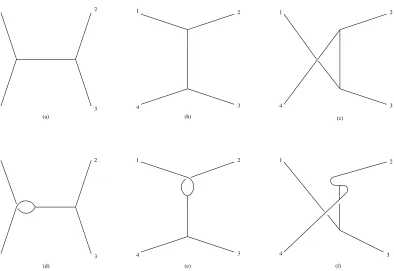
Using this conformal map Giddings managed to derive the Veneziano amplitude from CSFT. Because of the cubic vertex, in CSFT there are six relevant Feynman diagrams for four particles processes (fig.1). The contribution from the graph (a) in fig.1 was computed in [5] to be

As(p1, p2, p3, p4) =

Z 0

α0

dα2AG

dT

dα (β−α)

2(p1·p2+p3·p4)₍_β₊_α₎2(p1·p3+p2·p4)₍₂_α₎2(p2·p3)₍₂_β₎2(p1·p4)

(2.10) where the integration limitsα0 =

√

2₋1 andα = 0 correspond toT = 0 andT =_∞ respectively , 2AG is the ghost contribution and is given by

2AG = 8

1 2π

p

α2₊_γ2p_β2₊_γ2₍_β2

−α2)K(γ2) (2.11)

and the Jacobian factor almost cancels the ghost factor

dT dα =−

4(β2₋_α2₎

αAG

. (2.12)

2.2 Oscillator method: off-shell amplitude

Samuel derived a perturbative off-shell string amplitude [6] directly from string field theory by requiring that it reproduces Gidding’s result (2.10) when the momenta are set on-shell. We now briefly review Samuel results.

Let

g

2hV (3) 41I|hV

(3)

23J|b0e−T L0|VIJ(2)i= hV

(4)

1234| (2.13)

denote the vertex function associated with the graph (a) in fig.1, where the subscripts 1,2,3,4, I and J indicate Fock-space labels. The full contribution to the diagram is

Z ∞

0

dT_hV_1234||(4) Ψ(4)₄ _i|Ψ₃(3)_i|Ψ(2)₂ _i|Ψ(1)₁ _i (2.14)

where _|Ψ(rr)i is the Fock-space representation of the external states. The explicit

oscillator representations of _hV(2)_| _and _h_V(3)_|

hV12(2)|=

Z

d26p_hp_|(1)_{⊗ h}p_|(2)c(1)0 +c (2) 0

e−

P∞

n=1(−1)n

h

a(1)n ·a(2)n +cn(1)b(2)n +c(2)n b(1)n i

(2.15)

hV₁₂₃(3)_|=

Z

(10)

1 2

4 3

(a)

1 2

4 3

(b) (c)

1 2

4 3

(f) 4

1 ₂

3

(e) 1

4

2

3

(d)

1 2

[image:10.612.103.497.79.350.2]

4 3

Figure 1: The relevant Feynman diagrams for the four particles scattering.

·e−12

P3 r,s=1

h

a(mr)Vmnrsa

(s)

n +2a(mr)Vmrs0p(s)+p(r)V00rsp(s)−2c (r)

mXmnrs b

(s)

n i

(2.16)

show that all the terms in (2.14) are given in terms of exponentials of quadratic expressions in the oscillators. Using standard squeezed state techniques [9], closed-form expressions can be given for any perturbative amplitude. In the case of the four tachyon amplitude corresponding to the first diagram of fig.1, this procedure gives1

A4(p1, p2, p3, p4) =

λ2

cg2

2 δ(

P ipi)

R_∞

0 dT e

T _det1−( ˜X11₎2

1−( ˜V11₎2

e−12piQijpj (2.17)

where λc is a constant related to the Neumann coefficient for the three tachyon

vertex, λc =e3V

11 00 = 39/2

26 . In this formula ˜V11 and ˜X11 are defined by

˜

V_mn11 =e−(m+2n)TV11

mn X˜mn11 =e−

(m+n) 2 TX11

mn (2.18)

where Vrs _and _Xrs _{are infinite-dimensional matrices}

Vrs=

 

Vrs

11 V12rs . . . Vmnrs . . .

Vrs

21 V22rs . . . Vmrs+1,n . . .

. . . .



, Xrs =

 

Xrs

11 X12rs . . . Xmnrs . . .

Xrs

21 X22rs . . . Xmrs+1,n . . .

. . . .



 (2.19)

1

(11)

whose elements are matter and ghost Neumann coefficients of the cubic string field theory vertex, for which exact expressions are given in the Appendix A. Qij _are

defined as

Qij = V₀iI_m 1 1−( ˜V11₎2

mn

˜

V_np11V_pIj₀ +V₀₀11₋T(2₋δij) i, j = 1,2 ori, j = 3,4

Qij = ₋V0iIm

1 1−( ˜V11₎2

mn C

˜

Vnp11V Ij

p0 i= 1,2 andj = 3,4 ori= 3,4 andj = 1,2 (2.20)

where m, n, p _≥ 1, C = δmn(−1)n and the sum over I denotes a sum over the

intermediate states.

The two expressions (2.10) and (2.17) should both represent the contribution to the four tachyon amplitude coming from the diagram (a) in fig.1 when the momenta are on-shell. To relate them in the proper way, a general procedure was developed in [6] for computing the functions Qij _{appearing in (2.17) from the Giddings map,}

giving

Q11=Q44 = lnα₋lnκ, Q22 =Q33 =₋lnα₋lnκ Q12₌_Q21 ₌₋_ln_|_α₋_β_|_, _Q13 ₌_Q31 ₌₋_ln(_α₊_β₎

Q14=Q41 =₋ln(2β), Q23 =Q32 =₋ln(2α)

Q24=Q42 =₋ln(α+β), Q34 =Q43 =₋ln_|α₋β_| (2.21)

where κ is given as an integral

ln(κ) =₋2α√ (β2−α2) (α2₊_γ2₎₍_α2₊_δ2₎

R∞

1 dwln(w−1)

d dw

√

(w2₊_α2_γ2₎₍_w2₊_α2_δ2₎

(w+1)(β2_w2₋_α2₎

. (2.22)

As already noticed, althoughα, β, γ, δall appear in the above equation, there is only one independent variable, so that the functionκin (2.23) is actually a function of α. The substitution of (2.21) in (2.17) leads to the following formula

A4(p1, p2, p3, p4) = λ2c

g2 2 Z 0 α0 dαdT dαe

T_det1−( ˜X11₎2

1−( ˜V11₎2

[κ(α)]P4i=1p2i ₍_α₎−(p21+p24)+p22+p23

|α₋β_|2(p1·p2+p3·4)₍_β₊_α₎2(p1·p3+p2·4)₍₂_α₎2(p2·p3)₍₂_β₎2(p1·p4) _(2.23)

Comparing the two expressions (2.10) and (2.23) on shell (p2

i = 1), one can see that

the momentum dependence matches and for the momentum independent part the following identity holds

λ2_c

dT dα

eTdet1₁−₋( ˜_{( ˜}X_V1111₎)22

= 2Ag

dT dα

1

[κ(α)]4 . (2.24)

By trading the variableαfor the Koba-Nielsen variablexthrough (2.9) in (2.23), the contribution from the first graph in fig.1 becomes

A4(p1, p2, p3, p4) =

g2 2

Z 1

1 2

dx xp1·p2+p3·p4₍₁₋_x₎(p1+p4)2−2

κ(x) 2

P4_i₌₁p2_i−4

(12)

The remaining diagrams (b),(c),(d),(e),(f) of fig.1 can be obtained from the first one by a suitable permutation of the string labels, i.e. _{by permuting the momenta}

in (2.25), and the total four-point tachyon amplitude is the sum of these six contri-butions. Notice that the Veneziano amplitude is exactly reproduced when p2

i = 1 in

(2.25) and the additional factor containing κ(x) goes to 1.

2.3 Level truncation

The infinite-dimensional matrices (2.19) appearing in the final expression for a given diagram are expressed in terms of the Neumann coefficients of Witten’s vertex. The level truncation method we use in this paper consists in the truncation on the level of oscillators associated with the Neumann coefficients. This procedure is somewhat different from the original method of level truncation [4] (method a) section 1), in which one calculates the SFT action by only including in the string field expansion contributions up to a fixed total oscillator level. While the latter approach involves computations with a number of fields that grows exponentially in the level, in the for-mer one has to calculate the determinant of some matrices whose size grows linearly in the truncation level.

Let us explicitly remind the procedure [47] in the case of a tree diagram with four external fields as (2.17), in which there is a single internal propagator with Schwinger parameter T. One starts with a suitable change of coordinates in (2.17)

σ =e−T _(2.26)

then expands in powers of σ, so getting an expression of the form

Z 1

0

dσ σ2σ

p2X∞ n=0

cn(pi)σn =

∞

X n=0

cn(pi)

p2₊_n₋₁ , (2.27)

wherep=p1+p2 =p3+p4 represents the momentum of the intermediate state. The poles p2 _{= 1}₋_n _{in (2.27) clearly correspond to the contributions of intermediate} particles as the tachyon (n= 0), the gauge field (n = 1) and all the other open string massive fields. Truncate all the matrices to size L_×Lmeans to truncate the sum in (2.27) to n =L, thus imposing a limit on the mass of the intermediate states.

The analysis can be simplified by noting that in the four point amplitude the contributions of odd level fields cancel between s and t channels so that only even levels in the truncation, i.e. _{only even powers of} _σ _{in the expansion (2.27), need}

to be considered. An explicit example of the procedure above explained is given in Appendix B, where the four tachyon amplitude at level L = 2 is derived in the time-dependent case.

3. Solution for the function

κ

(

x

)

(13)

function κ(α, γ) we have first to solve eq.(2.3) for one of the two variables in terms of the other, so that the function κ will be a function of only one of the two α or

γ. Since the four point amplitude is written in terms of an integral over x, which is easily related to α through (2.9), it would be more natural to solve for γ as a function of α then the opposite. The solution can be found numerically and for γ

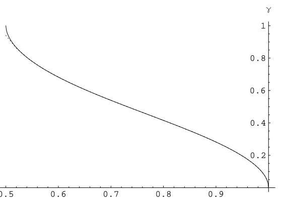
as a function of x is given by the solid line in fig.2. γ goes from 0 to 1 while x

goes from 1 to 1/2 and α goes from 0 to √2₋1. To check for the accuracy of the solution, we have found two different expansions: 1) A power series inα which gives

γ in a neighbor of 0 and can be inverted so as to give α as a function of γ around 0. 2) An expansion ofα around√2₋1 as an expansion in 1₋γ, this series cannot be inverted due to the presence of terms of the type (1₋γ)m_log(1₋_γ₎n_{. We have}

found a general procedure to obtain as many terms as necessary in both expansions and the function α(γ) can be determined in the whole range 0_≤γ _≤1. As we shall show in fact the two series for α(γ) overlap in an extended interval that goes from

γ _∼0.6 to γ _∼0.7.

3.1 γ and α around 0

By using the integral representations of the elliptic functions [46] it is possible to write the equation (2.3) in a useful form

E(γ2)

Z γ/α

αγ

dtp 1

t2₊_γ4√_{1 +}_t2 −(1−γ

4₎_K₍_γ2₎

Z γ/α

αγ

dtp 1

t2₊_γ4₍√_{1 +}_t2₎3 =

π

4 (3.1) To expand (3.1) for small γ andαwe have to divide the integration region into three intervals in such a way that the square roots in the denominators of (3.1) can be consistently expanded and the integrals in t performed. For example consider the integral in the first term of (3.1), it can be rewritten as

Z γ/α

αγ

dtp 1

t2₊_γ4√_{1 +}_t2 =

Z γ2

αγ

dt 1

γ2q_{1 +} t2

γ4

√ 1 +t2

+

Z 1

γ2

dt 1

t

q

1 + γ_t24

√ 1 +t2

+

Z γ_α

1

dt 1

t2q_{1 +} γ4

t2

q

1 + _t12

(3.2)

In each integral of the rhs the integration domain is contained in the convergence radius of the Taylor expansions of the square roots containing γ, so that they can be safely expanded and the integrals in t performed.

With this procedure one gets the following equation equivalent to (3.1)

E(γ2) ∞

X n,k=0

Γ(1₂)2

(14)

(

2 2n+ 2k+ 1

"

γ4k₋

α γ

2n+1

(αγ)2k

#

+ (1₋δkn)

γ4n₋_γ4k

2k₋2n −δknγ

4n_ln_γ2

)

−(1₋γ4)K(γ2) ∞

X n,k=0

Γ(1 2)Γ(−

1 2) Γ(1

2 −n)Γ(− 1

2 −k)n!k!

(

1 2n+ 2k+ 1

"

γ4k₋

α γ

2n+1

(αγ)2k

#

+ (1₋δkn)

γ4n₋γ4k

2k₋2n −δknγ

4n_ln_γ2

+ 1

2n+ 2k+ 3

"

γ4n₋

α γ

2k+3

(αγ)2n

#)

= π

4 (3.3)

The series containing lnγ2 _{can be resummed, the first gives} 2

πK(γ

2_{) the second} 2

π(1−γ4₎E(γ2). Hence these terms cancel and lnγ2 actually disappears from the

equa-tion. As a consequence one can write γ as a power series in α whose coefficients are determined requiring that eq.(3.3) is satisfied. γ turns out to contain only the powers α4n+1_, _n _∈ _N_{. We have determined the first 12 terms of this series to get a} very good approximation for γ in an extended neighbor of zero (in which sense it is an extended neighbor will be clarified later)

γ =√3α

1 + 5α4+ 1041 16 α

8₊ 38719 32 α

12₊109062913 4096 α

16₊5278728465 8192 α

20₊

2172202186251 131072 α

24₊116561474500179 262144 α

28₊3303689940814193505 268435456 α

32₊

187301165958864015157 536870912 α

36₊ 86571446884950765378149 8589934592 α

40₊

5078927050639748451791733 17179869184 α

44

+ O(α48)

(3.4)

Any higher order in (3.4) can be in principle computed from (3.3). Using (2.9) we can plot γ as a function of x and compare it to the graph obtained from the numerical solution of eq.(3.1). As it is clear from fig.2 γ(x) has in x = 1/2 a vertical tangent, thus showing the presence of a branch point which cannot be gotten from a power series of the form (3.4). Nevertheless (3.4) gives a very good approximation forγ(x) except in a small neighbor of x = 1/2. In particular the agreement between the values of γ obtained from the series (3.4) and the numerical values is on the 15-th significative digit for 0.8 _≤ x _≤ 1, where the series (3.4) is expected to give exact results, thus providing a precision test for the accuracy of the numerical solution. Moreover, the expansion (3.4) can be iteratively inverted to give a series for α as a function of γ

α = _√γ 3

1₋ 5 9γ

4₊ 959 1296γ

8

− 10993₇₇₇₆ γ12+ 83359631 26873856γ

16

− 3579242677_483729408 γ20+ 1297273056905

69657034752 γ

24₋ 6783253984031 139314069504 γ

28₊168109910408625655 1283918464548864 γ

32₋

24949101849547687507 69331597085638656 γ

36₊10046339553062261150885 9983749980331966464 γ

(15)

[image:15.612.154.435.81.285.2]

0.5 0.6 0.7 0.8 0.9 x 0.2 0.4 0.6 0.8 1 Γ

Figure 2: Plots of γ(x): the solid line is the numerical solution of the elliptic equation, the dashed line is the power series.

512861712698825472832315 179707499645975396352 γ

44₊_O₍_γ48₎

(3.5)

By plugging the expansion (3.4) in (2.22) and using (2.9), the corresponding expan-sion for κ(α) can be found by means of numerical integration

κ(α) = 8 3√3 exp

−2.5α4₋7.1562α8₋75.927α12₋1238.7α16₋24301α20

−531290α24₋1.2489_·107α28₋3.0923_·108α32

−7.9627_·109α36₋2.1140_·1011α40₋5.7517_·1012α44

+O(α48).

(3.6)

3.2 γ around 1 and α around √2₋1

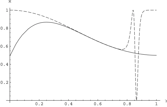
Around x = 1/2, i.e _α ₌ √₂₋_{1 and} _γ _{= 1, it is possible to obtain only} _x _(or _α₎

as a function ofγ and not the opposite. Such an expansion can be obtained by first expanding eq.(3.1) aroundγ = 1 and then looking for an expansion of α in terms of powers of 1₋γ and ln(1₋γ)

α=√2₋1 +a1(1−γ) +a2(1−γ)2+· · ·+b1(1−γ) ln(1−γ)+

b2(1−γ)2ln(1−γ) +· · ·+c1(1−γ)(ln(1−γ))2+c2(1−γ)2(ln(1−γ))2+. . . (3.7)

The coefficients in (3.7) are determined by requiring that (3.1) is satisfied. We provide here directly the expansion of x as a function of 1₋γ up to the ninth order

x= 1 2 +

1

8(1−γ) 2

1₋2 log 1−₄γ

− 1₄(1₋γ)3log 1−₄γ

(16)

0.2 0.4 0.6 0.8 1 Γ 0.2

[image:16.612.151.442.88.275.2]

0.4 0.6 0.8 1 x

Figure 3: Plots of x(γ): the dashed line gives the expansion of x(γ) which holds in a neighbor of γ = 1, the solid line gives the expansion of x(γ) aroundγ = 0.

1

16(1−γ) 4

1 + 3 log 1−₄γ

− ₉₆1 (1₋γ)5

7 + 12 log 1−₄γ

+ 1

1536(1−γ) 6

−97₋108 log 1−γ

4

−24 log2 1−γ

4

+ 64 log3 1−γ

4

− 1

2560(1−γ) 7

119 + 100 log 1−₄γ

−40 log2 1−₄γ

−320 log3 1−₄γ

+ 1

10240(1−γ) 8

−321₋60 log 1−₄γ

+ 1240 log2 1−₄γ

+ 2240 log3 1−₄γ

+ 1

107520(1−γ) 9

−1871 + 5740 log 1−₄γ

+ 29120 log2 1−₄γ

+ 31360 log3 1−₄γ

+. . .

(3.8)

From (3.5) one can easily getxas a function of γ in the regionx_∼1 (γ _∼0) so that x(γ) can be obtained for the whole range 1/2_≤x _≤1. The two expansions in fact overlap in a long range for 0.3 _≤γ _≤ 0.7 as it is shown in fig.3. They have an excellent agreement up to the 13-th significative digit for 0.6_≤γ _≤0.7.

4. Coefficient of the Quartic Tachyon Potential

The static tachyon potential has the form2

VT =

1 2φ

2

−g k φ3+g2k2c4φ4+. . . (4.1)

where g is the string coupling constant and k= 37/2

27 .

The four point tachyon potential is obtained from the off-shell four tachyon amplitude by setting to zero the external momenta and by explicitly subtracting out

2

(17)

the term with the tachyon on the internal line. The amplitude is the sum of the six Feynman diagrams shown in fig.1, the first of which gives the contribution (2.25) that can be usefully rewritten in terms of the Mandelstam variables

A4(s, t, u) = g 2_λ2

c

2

Z 1

1 2

dx xt−s2−u(1−x)s−2

κ(x) 2

t+s+u−4

. (4.2)

To get explicitly the first diagram contribution to the amplitude one can sett=u= 0 in (4.2), A4 can then be defined through an analitical continuation of (4.2) to the region s _≤ 1. This can be achieved by adding and subtracting the pole in x = 1 in the integrand of (4.2)

Z 1

1 2

dx x−s2(1−x)s−2

κ(x) 2

s−4

=

Z 1

1 2

dx x−s2(1−x)s−2

"

κ(x) 2

s−4

−

κ(1) 2

s−4#

+

κ(1) 2

s−4Z 1

1 2

dx x−s2(1−x)s−2 . (4.3)

where the first integral is now well defined ins= 0. When Re_[_s_]_>_{1 the last integral}

in (4.3) gives

2s−2 √

πΓ(1− s

2)Γ(

s

2 − 1 2) +

22−2s s₋2 2F1

1,2₋s; 2₋ s 2;−1

that has a well defined limit for s_→0, so that the four point tachyon potential can be written

A4(0,0,0) = g 2_λ2

c 2 " Z 1 1 2 dx 2

κ(x)

4 − 2 κ(1) 4!

(1₋x)−2 − 3₂

2

κ(1)

4#

(4.4)

As already pointed out, the function κ(x) in (4.4) can be evaluated numerically in the whole interval 1

2 < x < 1, by using the numerical solution of eq.(3.1) graphed in fig.??. The integrand in (4.4) is regular atx= 1, as can be easily checked by studying the behavior of (3.6) in a neighbor of α= 0. However, problems are expected in the numerical evaluation of the integral in a neighbor of x= 1 due to the product of a pole times a zero. To circumvent possible computational problems we divided the interval 1₂ < x < 1 into two parts . For x _∈ [1₂,0.95] we used numerical evaluation of κ(x), by plugging the numerical solutions of (3.1) in (2.22). For x _∈ [0.95,1] we used the analitical expression obtained substituting (2.9) in (3.6). By summing the two contributions we have found the value A4(0,0,0) = ₋g₂22.94497480(2). To get the the quartic term of the tachyon effective potential we have to subtract [4] from (4.4) the contribution from the internal tachyon line

A4t(s, t, u) =

g2 2 λ

2−s−t+3u

c

1

(18)

evaluated at s= t =u= 0. Each graph in fig.1 contributes equally, so that for the quartic tachyon coupling one eventually gets

g2k2c4 = 6

4![A4(0,0,0)−A4t(0,0,0)] = 6 4!

g2

2(−2.94497480(2)+ 39 212) =

g2

4! 5.5813353(1) (4.6) where the factor 1/4! is required to recover the units of [48, 10]. The numerical evaluation of the coefficientc4from the exact four tachyon amplitude was given in [6] to an accuracy of 1%,c4 ≈1.75(2), and in [10] to an accuracy of 0.1%,c4 ≈1.742(1). We have repeated this calculation to an higher degree of precision, and the result (4.6) gives

c4 ≈1.74220008(3). (4.7)

This coefficient was calculated using the level truncation scheme up to level L = 20 in [48], and improved up to level L= 28 in [13], thus obtaining c4,L=28≃ −1.70028, with a discrepancy of 2.4% with respect to (4.7). In the same paper, a procedure to extrapolate the known level truncated results and predict the asymptotic L _{→ ∞}

value for c4 was described, giving an extimated value c4,L→∞ = 1.7422006(9) that agrees within the 10−7 _{of accuracy with our exact result (4.7).}

5. The rolling tachyon in cubic string field theory

As a second application of the formalism developed in Section 2, we discuss some properties of the rolling tachyon solutions in CSFT. This problem has been faced analytically in [20] at the (0,0) level, and numerically in [18, 19, 14]. In particular, a level truncated analysis of the tachyon dynamics was carried out in [14] for a perturbative solution given as a sum of exponentials of the form

φ(t) =X

n>0

anent . (5.1)

The solution and all its derivatives satisfy the boundary conditionφ _→0 ast_{→ −∞}. The coefficients in (5.1) can be determined by perturbatively solving the CSFT equation of motion. For such a profile the φn+1 _{term in the tachyon effective action} contributes only to the coefficients ak with k ≥ n. Since in the CSFT tachyon

effective action

S[φ] =X

n

gn−2

n!

Z n

Y i=1

(2πdki)δ( X

i

ki)φ(k1). . . φ(kn)An(k1, . . . , kn) (5.2)

the coefficients A2 and A3 are exactly known,

A2(k1, k2) = 1−k1k2 , A3(k1, k2, k3) = −2

3√3 4

!3+k21+k22+k23

(19)

the first two coefficients in (5.1) are exact and can be normalized as a1 = 1, a2 = −64/(243√3).

In [14] an L = 2 approximation was explicitly provided for the coefficients

a3. . . a6 in the sum (5.1)

φ(t)∼=et₋ 64

243√3e

2t₊₀_.₀₀₂₁₈₇_e3t

−3.9258 10−6_e4t₊₄_._{9407 10}−10_e5t

−6.3227 10−12_e6t

(5.4) For negativetEq.(5.4) describes the rolling of the tachyon off the unstable max-imum along the potential. The physical interpretation for positive t is more prob-lematic. The truncated expansion (5.4) is a solution only up to some upper bound

t = tb which increases by increasing the number of terms one includes in the sum.

Consequently, the asymptotic behavior of the solution for large positive t cannot be extrapolated from Eq.(5.4), being the sum alternate the asymptotic behavior would simply be _±∞ depending on the order n at which one truncates the sum (5.1).

Before exponentially exploding φ(t) presents an oscillatory behavior with in-creasing amplitudes that makes the rolling tachyon dynamics in the framework of CSFT for positive t difficult to interpret. In ref. [14], however, it was shown that the trajectory φ(t) is well-defined. Increasing both the level of truncation and the number of terms retained in the power series (5.1) leads to a convergent value ofφ(t) for any fixed t with t < tb. If the position of the first turnaround points, that the

solution exhibits fort >0, tends to stabilize as the truncation levelLof the effective actions increases, the expansion (5.4) fort > 0 would be justified at least up to those points. The trajectories φ(t), obtained by computing the φ4 term in the effective action up to L = 16, show that indeed the position of the first two turnaround points seems to stabilize [14]. Fort >0, the tachyon does not roll towards the stable non-perturbative minimum of the potential.

We shall now study how this solution is modified by using the exact value of the 4-tachyon term in the effective action for homogeneous time dependent profiles. The exact value of the coefficient a3 can be obtained by computing integrals of the type (2.25), that in the time-dependent case read

A4(p1, p2, p3, p4) =

g2 2

Z 1

1 2

dx x−p1·p2−p3·p4₍₁₋_x₎−(p1+p4)2−2

κ(x) 2

−P4_i₌₁p2_i−4

(5.5)

To get the equations of motion the function A4 in (5.2) has to be evaluated for imaginary integer values of the field modes so that (5.5) is regular and does not need any analytical continuation. In the evaluation of a3, the relevant integral (5.5) over the Kobe-Nielsen variable is

A4(−i,−i,−i,3i) =

g2 2

Z 1

1 2

dx x−2₍₁ −x)2

κ(x) 2

8

(20)

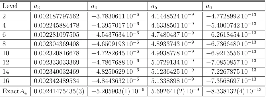
Summing all the diagrams in fig.1 and subtracting the corresponding contributions coming from the internal tachyon line, A4t = 229/322, we get a3 = 0.00241475435(3). This value, which is exact, can be compared with the corresponding ones obtained through the level truncation approximation. The first column of Table 1 shows the

Level a3 a4 a5 a6

2 0.002187797562 ₋3.7830611 10−6 ₄_._{1448524 10}−9 ₋₄_._{7728992 10}−13 4 0.002245884478 ₋4.3957017 10−6 ₄_._{6338501 10}−9 ₋₅_._{4000742 10}−13 6 0.002281097505 ₋4.5437634 10−6 ₄_._{7480437 10}−9 ₋₆_._{2618454 10}−13 8 0.002304369408 ₋4.6509193 10−6 ₄_._{8933743 10}−9 ₋₆_._{7366480 10}−13 10 0.002320816678 ₋4.7282645 10−6 ₄_._{9938778 10}−9

[image:20.612.85.552.166.337.2]

−6.9213556 10−13 12 0.002333033369 ₋4.7867688 10−6 ₅_._{0729134 10}−9 ₋₇_._{0850857 10}−13 14 0.002340032469 ₋4.8250629 10−6 ₅_._{1236425 10}−9 ₋₇_._{2267875 10}−13 16 0.002342489534 ₋4.8443632 10−6 ₅_._{1338898 10}−9 ₋₇_._{3568697 10}−13 ExactA4 0.00241475435(3) −5.205903(1) 10−6 5.692641(2) 10−9 −8.338132(4) 10−13

Table 1: First few coefficients an of the time-dependent solution

P

nane nt

at various levels of truncation, when only the contribution from the quartic term in the effective action is considered in the EOM. In the last row the exact four tachyon amplitude is used for the calculations.

sequence of the first approximate values of thea3(L) coefficients up to L= 14. The level sequence is perfectly consistent with the exact value given in the last row (first column), which should then be considered as the limit a3(L→ ∞).

The amplitude (2.25) can be used to improve the accuracy of the remaining coefficients an, n ≥ 4. The exact evaluation of a4 would require the knowledge of

A5(p1, . . . , p5), for which an expression analog to (2.25) is not known. However, when solving the CSFT equation of motion, one can easily see that the dominant contribution to a4 comes from the lower order amplitudes A2(p1, p2), A3(p1, p2, p3),

A4(p1, p2, p3, p4). Therefore, for a precise evaluation of a4 seems more relevant to know these lower order amplitudes exactly, rather than A5(p1, . . . , p5) approximate in levels. The remaining columns in Table 1 give the behavior of the coefficients a4,

a5,a6 for increasing levels of truncation, when only the contribution from the quartic term in the effective action is considered in the equations of motion. The last row gives the corresponding value obtained from the exact amplitude (2.25) (i.e. _limit

L _{→ ∞}). As can be seen from Table 1, for any fixed L, _|an(L)| < |an(L → ∞)|.

Notice that the same property holds also in the calculation of the coefficient of the quartic tachyon potential. Indeed, up toL= 28 [13], _|c4,L|<|c4|. Moreover, for any fixed n, the sequence (an(L+ 2)−an(L)) goes likeCnan(L)/L,Cn being a constant,

(21)

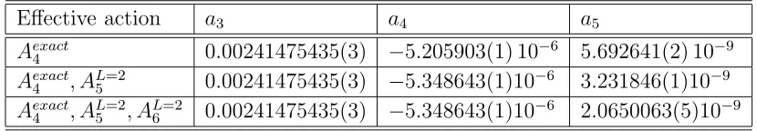
We can now include in the computation of a4, a5, a6 the L = 2 truncated ex-pressions forA5(p1, . . . , p5), A6(p1, . . . , p6), A7(p1, . . . , p7). The numerical results are listed in Table 2. The L= 2 truncated A7(p1, . . . , p7), however, gives a contribution to a6 which is not reliable, since increasing the order of the effective action higher level field components become more and more important. The inclusion of the a6 coefficient, in any case, does not change the behavior of the solution around the first two turnaround points. This is the region where we shall mainly focus, only here the solution with the first few coefficients is reliable.

Effective action a3 a4 a5

Aexact

4 0.00241475435(3) −5.205903(1) 10−6 5.692641(2) 10−9

Aexact

4 , AL5=2 0.00241475435(3) −5.348643(1)10−6 3.231846(1)10−9

Aexact

[image:21.612.90.505.222.294.2]

4 , AL5=2, AL6=2 0.00241475435(3) −5.348643(1)10−6 2.0650063(5)10−9

Table 2: First few coefficients an of the time-dependent solution

P

nane nt

. The first column indicates which terms of the effective action are considered in the EOM.

In fig.4 we show how the solution changes at the second turnaround point by in-troducing higher order terms of the effective action. The higher group of trajectories is obtained by using the exact value for the four-tachyon effective action and adding to it the level L = 2 five and six tachyon effective action, the lower group by using only L = 2 terms (the solid line in this group represent the solution of ref. [14] up to thee5t _{power). As it is manifest from the figure the use of an exact} _A

4 leads to a decreasing of the amplitude of the oscillations by at least the 20%. This is however not enough to change the qualitative behavior of the solutions which maintains huge oscillations and does not provide a physically meaningful picture. The best approx-imation we get is given by the solution obtained using the exact A4 and the level 2

A5, A6. It reads

φ(t)∼=et₋ 64

243√3e

2t_{+ 0}_._00241475_e3t

−5.34864310−6e4t+ 2.065006310−9e5t (5.7)

and is plotted in fig.5 against the solution (5.4) of ref. [14] up to the coefficient of

e5t_.

The solution (5.7) can also be compared to the analytic solution found in [20] at the (0,0) level that reads, for t <0,

φ(t) =₋6λ−53

c

∞

X n=1

−1 6

n

nλ−43n2+3n

c ent , (5.8)

where λc = 3

9

2/26. In [20], a different expression was considered for t > 0. If

(22)

3.4 3.6 3.8 4.2

[image:22.612.160.438.80.262.2]

-80 -60 -40 -20

Figure 4: Solution at the second turnaround point. The higher group of trajectories is obtained by using the exact value for the four-tachyon effective action (solid line) and adding to it the levelL= 2 five (long dashed line) and six (dashed line) tachyon effective action, the lower group by using only L = 2 terms. The solid line in the lower group represents the solution of ref. [14] up to thee5t power.

compared to (5.7) and (5.4). For t < 0 all the solutions overlap up to the 6-th significative digit. For positive t, all the solutions present the expected oscillatory behavior with ever-growing amplitudes and have constant energy. In CSFT where the action contains infinite derivatives the kinetic energy can be negative and thus the tachyon can move to higher and higher heights on the tachyon potential while conserving the total energy [18]. Whatever solution one chooses, the position of the first extremum seems to be fixed at t1 ∼ 1.27 with amplitude φ(t1) ∼ 1.74. In addition, such a position is compatible within the 1% also with [18], where an analog approximate solution was considered using the coshnt basis. This suggests the idea that the first maximum could have a physical meaning. Actually, since the solution describes the motion of the tachyon rolling off its unstable maximum at φ = 0, the naive energy conservation would confine the motion between 0 _≤φ(t)_≤φM, where

φM denotes the maximum value attained byφi.e. is the naive inversion point defined

by the conditionVef f[0] =Vef f[φM] on the effective tachyon potentialVef f. A natural

interpretation for the first maximum is thereforeφ(t1)∼φM. Numerically, the value

φM ∼1.7 is in fact in a qualitative agreement with the available data on the effective

tachyon potential [50].

(23)

3.4 3.6 3.8 4.2

[image:23.612.176.421.81.237.2]

-80 -60 -40 -20

Figure 5: Second turnaround point for the solution (solid line) given in ref. [14] and the solution (dashed line) obtained using the exact A4 and the level 2A5,A6.

one by an order of magnitude.

In conclusion, it seems that up to the first turnaround point all the solutions (5.4), (5.7), (5.8), practically coincide. After the first turnaround point, the wild oscillations with increasing amplitudes found in refs.[18, 14] are confirmed. Although the qualitative behavior is reproduced, the oscillations in (5.7) are sensibly reduced when compared to those in ref.[14]. Up to the second turnaround point, where low powers of et _{dominate, (5.7) provides a more accurate estimate for the trajectory of}

the rolling tachyon in CSFT.

Acknowledgments

We are grateful to E. Coletti, W. Taylor and I. Sigalov for useful discussions.

A. Neumann Coefficients

Exact formulas for the Neumann coefficients Vrs _and _Xrs _{appearing in (2.19) were}

computed in [51]3_{. The indices}_{r, s}_{take values from 1-3 and indicate wich Fock space} the oscillators act in. The 3-string coefficients Vrs

mn, Xmnrs are given in terms of the

3

(24)

6-string Neumann coefficients Nr,±s nm

Nr,±r nm =

(

1

3(n±m)(−1)

n₍_A

nBm±BnAm), m+neven, m6=n

0, m+nodd (A.1)

N_nmr,±(r+σ) =

( ₁

6(n±σm)(−1)

n+1₍_A

nBm±σBnAm), m+neven, m6=n

σ₆₍_n√_±3_σm₎(AnBm∓σBnAm), m+nodd

#

.

(A.2)

where inNr,±(r+σ)_, _σ ₌_±_{1, and} _r₊_σ _{is taken modulo 3 to be between 1 and 3. In} (A.2) An, Bn are defined for n ≥0 through

1 +ix

1₋ix

1/3

= X

neven

Anxn+i X modd

Amxm (A.3)

1 +ix

1₋ix

2/3

= X

neven

Bnxn+i X modd

Bmxm.

The 3-string matter Neumann coefficients Vrs

nm are then given by

V_nmrs =₋√mn(N_nmr,s +N_nmr,−s), m₆=n, andm, n₆= 0

V_nnrr =₋1 3 " 2 n X k=0

(₋1)n−kA2_k₋(₋1)n₋A2_n

#

, n₆= 0

V_nnr,r+σ = 1 2[(−1)

n

−V_nnrr], n₆= 0 (A.4)

V₀rs_n =₋√2n N₀r,s_n +N₀r,_n−s

, n ₆= 0

V₀₀rr = ln(27/16) The ghost Neumann coefficients Xrs

mn, m≥0, n >0 are given by

X_mnrr = m ₋N_nmr,r +Nr,−r nm

, n ₆=m X_mnr(r±1) = m _±N_nmr,r∓1_∓N_nmr,−(r∓1)

, n₆=m (A.5)

X_nnrr = 1 3

"

−(₋1)n₋A2_n+ 2

n X

k=0

(₋1)n−k_A2

k−2(−1)nAnBn #

Xr(r±1)

nn = −

1 2(−1)

n

− 1₂X_nnrr

The Neumann coefficients satisfy a cyclic symmetry under r _→ r + 1, s _→ s + 1, corresponding to the geometric symmetry of rotating the vertex. Furthermore, they are symmetric under the exchange r _↔ s, n _↔ m and satisfy the twist symmetry associated with reflection of the strings

Vrs

nm = (−1)n+mVnmsr (A.6)

(25)

B. Level truncation method

As a specific example of the level truncation method explained in Section 2.3 let us derive explicitly the four tachyon amplitude for L = 2 in the time-dependent case. At this level of truncation and with the change of coordinates (2.26), the matrices

˜

V11 _{and ˜}_X11 _{in (2.17) become the 2}_×_{2 matrices}

˜

V11₌ V 11

11σ V1211σ

3 2 V11

21σ

3 2 V11

22σ2

!

, X˜11₌ X 11

11σ X1211σ

3 2 X11

21σ

3 2 X11

22σ2

!

(B.1)

and analog forms for all the objects contained in (2.20) may be written. Expanding the determinant and the exponential in (2.17) in powers of σ up to σ2 _{one gets}

A4(p1, p2, p3, p4) =

λ2

cg2

2 λ

2 3(

P4

i=1p2i+p1·p2+p3·p4)

c δ(

X i

pi)

Z 1

0

dσ σ2σ

−1₂[(p1+p2)2+(p3+p4)2]

1₋b1(p1−p2)(p3−p4)σ+ 1 2

b2 +b3 (p1−p2)2+ (p3−p4)2

+b4(p1−p2)2(p3−p4)2+b5(p1+p2)(p3+p4)

σ2+O(σ3) (B.2)

where

b1 = (V0112)2, b2 = 26(V1111)2−2(X1111)2, b3 = (V0112)2V1111,

b4 = (V0112)4, b5 = 18(V0212)2. (B.3)

To get the quartic term in the tachyon effective action on has to subtruct the con-tribution from the tachyon in the propagator, that corresponds to the σ0 _{power -the} constant term 1- in (B.2). Since, as already noticed, for a four point amplitude only even powers of σ need to be considered, one is left with the coefficient of the σ2 term in the sum. Performing the integral over σ, one finally gets the formula for the quartic term in the CSFT tachyon effective action (5.2) in the time-dependent case

AL₄=2(p1, p2, p3, p4) = λ2cg2

Z n

Y i=1

(2πdpi)δ( X

i

pi)φ(pi)

λ23(

P4

i=1p2i+p1·p2+p3·p4)

c

1₋(p1+p2)2

b2

4 +b3p1(p2−p1) +b4p2p4(p2−p1)(p4−p3) +b5p2p4

(B.4)

References

[1] E. Witten, “Noncommutative Geometry And String Field Theory,” Nucl. Phys. B 268, 253 (1986).

(26)

[3] W. Taylor, “Perturbative computations in string field theory,” arXiv:hep-th/0404102.

[4] V. A. Kostelecky and S. Samuel, “The Static Tachyon Potential In The Open Bosonic String Theory,” Phys. Lett. B 207, 169 (1988).

[5] S. B. Giddings, “The Veneziano Amplitude From Interacting String Field Theory,” Nucl. Phys. B278, 242 (1986).

[6] S. Samuel, “Covariant Off-Shell String Amplitudes,” Nucl. Phys. B308, 285 (1988).

[7] J. H. Sloan, “The Scattering Amplitude For Four Off-Shell Tachyons From Functional Integrals,” Nucl. Phys. B 302, 349 (1988).

[8] S. Samuel, “Solving The Open Bosonic String In Perturbation Theory,” Nucl. Phys. B341, 513 (1990).

[9] V. A. Kostelecky and R. Potting, “Analytical construction of a nonperturbative vacuum for the open bosonic string,” Phys. Rev. D 63, 046007 (2001)

[arXiv:hep-th/0008252].

[10] W. Taylor, “Perturbative diagrams in string field theory,” arXiv:hep-th/0207132.

[11] I. Bars and I. Y. Park, “Improved off-shell scattering amplitudes in string field theory and new computational methods,” Phys. Rev. D 69, 086007 (2004) [arXiv:hep-th/0311264].

[12] I. Bars, “MSFT: Moyal star formulation of string field theory,” arXiv:hep-th/0211238.

[13] M. Beccaria and C. Rampino, “Level truncation and the quartic tachyon coupling,” JHEP 0310, 047 (2003) [arXiv:hep-th/0308059].

[14] E. Coletti, I. Sigalov and W. Taylor, “Taming the tachyon in cubic string field theory,” JHEP0508, 104 (2005) [arXiv:hep-th/0505031].

[15] A. Sen, “Rolling tachyon,” JHEP 0204, 048 (2002) [arXiv:hep-th/0203211].

[16] A. Sen, “Time evolution in open string theory,” JHEP0210, 003 (2002) [arXiv:hep-th/0207105].

[17] F. Larsen, A. Naqvi and S. Terashima, “Rolling tachyons and decaying branes,” JHEP 0302, 039 (2003) [arXiv:hep-th/0212248].

[18] N. Moeller and B. Zwiebach, “Dynamics with infinitely many time derivatives and rolling tachyons,” JHEP 0210, 034 (2002) [arXiv:hep-th/0207107].

[19] M. Fujita and H. Hata, “Time dependent solution in cubic string field theory,” JHEP 0305, 043 (2003) [arXiv:hep-th/0304163].

(27)

[21] J. A. Minahan, “Rolling the tachyon in super BSFT,” JHEP0207, 030 (2002) [arXiv:hep-th/0205098].

[22] M. R. Gaberdiel and M. Gutperle, “Remarks on the rolling tachyon BCFT,” arXiv:hep-th/0410098.

[23] A. Sen, “Dirac-Born-Infeld action on the tachyon kink and vortex,” Phys. Rev. D 68, 066008 (2003) [arXiv:hep-th/0303057].

[24] D. Kutasov and V. Niarchos, “Tachyon effective actions in open string theory,” Nucl. Phys. B 666, 56 (2003) [arXiv:hep-th/0304045].

[25] M. R. Garousi, “Slowly varying tachyon and tachyon potential,” JHEP0305, 058 (2003) [arXiv:hep-th/0304145].

[26] A. Fotopoulos and A. A. Tseytlin, “On open superstring partition function in inhomogeneous rolling tachyon background,” JHEP0312, 025 (2003)

[arXiv:hep-th/0310253].

[27] A. Strominger, “Open string creation by S-branes,” arXiv:hep-th/0209090.

[28] M. Gutperle and A. Strominger, “Timelike boundary Liouville theory,” Phys. Rev. D 67, 126002 (2003) [arXiv:hep-th/0301038].

[29] F. Leblond and A. W. Peet, “SD-brane gravity fields and rolling tachyons,” JHEP 0304, 048 (2003) [arXiv:hep-th/0303035].

[30] A. Strominger and T. Takayanagi, “Correlators in timelike bulk Liouville theory,” Adv. Theor. Math. Phys. 7, 369 (2003) [arXiv:hep-th/0303221].

[31] V. Schomerus, “Rolling tachyons from Liouville theory,” JHEP 0311, 043 (2003) [arXiv:hep-th/0306026].

[32] J. McGreevy and H. L. Verlinde, “Strings from tachyons: The c = 1 matrix reloaded,” JHEP 0312, 054 (2003) [arXiv:hep-th/0304224].

[33] I. R. Klebanov, J. Maldacena and N. Seiberg, “D-brane decay in two-dimensional string theory,” JHEP 0307, 045 (2003) [arXiv:hep-th/0305159].

[34] N. R. Constable and F. Larsen, “The rolling tachyon as a matrix model,” JHEP 0306, 017 (2003) [arXiv:hep-th/0305177].

[35] J. McGreevy, J. Teschner and H. L. Verlinde, “Classical and quantum D-branes in 2D string theory,” JHEP 0401, 039 (2004) [arXiv:hep-th/0305194].

[36] T. Takayanagi and N. Toumbas, “A matrix model dual of type 0B string theory in two dimensions,” JHEP 0307, 064 (2003) [arXiv:hep-th/0307083].

(28)

[38] I. Y. Aref’eva, L. V. Joukovskaya and A. S. Koshelev, “Time evolution in superstring field theory on non-BPS brane. I: Rolling tachyon and

energy-momentum conservation,” JHEP 0309, 012 (2003) [arXiv:hep-th/0301137].

[39] M. Fujita and H. Hata, “Rolling tachyon solution in vacuum string field theory,” Phys. Rev. D 70, 086010 (2004) [arXiv:hep-th/0403031].

[40] L. Bonora, C. Maccaferri, R. J. Scherer Santos and D. D. Tolla, “Exact

time-localized solutions in vacuum string field theory,” Nucl. Phys. B 715, 413 (2005) [arXiv:hep-th/0409063].

[41] L. Bonora, C. Maccaferri, R. J. Scherer Santos and D. D. Tolla, “Fundamental strings in SFT,” Phys. Lett. B 619, 359 (2005) [arXiv:hep-th/0501111].

[42] T. Lee and G. W. Semenoff, “Fermion representation of the rolling tachyon

boundary conformal field theory,” JHEP 0505, 072 (2005) [arXiv:hep-th/0502236].

[43] E. Coletti, V. Forini, G. Grignani, G. Nardelli and M. Orselli, “Exact potential and scattering amplitudes from the tachyon non-linear beta-function,” JHEP 0403, 030 (2004) [arXiv:hep-th/0402167].

[44] G. W. Gibbons, “Cosmological evolution of the rolling tachyon,” Phys. Lett. B537, 1 (2002) [arXiv:hep-th/0204008].

[45] G. Calcagni, “Cosmological tachyon from cubic string field theory,” arXiv:hep-th/0512259.

[46] I. S. Gradshteyn and I. M. Ryzhik , “Table of Integrals, Series, and Products,” Academic Press (2000).

[47] E. Coletti, I. Sigalov and W. Taylor, “Abelian and nonabelian vector field effective actions from string field theory,” JHEP 0309, 050 (2003) [arXiv:hep-th/0306041].

[48] W. Taylor, “D-brane effective field theory from string field theory,” Nucl. Phys. B 585, 171 (2000) [arXiv:hep-th/0001201].

[49] W. Taylor, “A perturbative analysis of tachyon condensation,” JHEP 0303, 029 (2003) [arXiv:hep-th/0208149].

[50] N. Moeller and W. Taylor, “Level truncation and the tachyon in open bosonic string field theory,” Nucl. Phys. B 583, 105 (2000) [arXiv:hep-th/0002237].

[51] D. J. Gross and A. Jevicki, “Operator Formulation Of Interacting String Field Theory. 2,” Nucl. Phys. B 287, 225 (1987).