Article
Nonlocal Tensor Sparse Representation and
Low-Rank Regularization for Hyperspectral Image
Compressive Sensing Reconstruction
Jize Xue 1, Yongqiang Zhao2,* , Wenzhi Liao3 and Jonathan Cheung-Wai Chan4
1 School of Automation, Northwestern Polytechnical University, Xi’an 710072, China;
2 Research & Development Institute of Northwestern Polytechnical University in Shenzhen,
Shenzhen 518057, China
3 Department of Telecommunications and Information Processing, Ghent University-TELIN-IMEC,
9000 Ghent, Belgium; [email protected]
4 Department of Electronics and Informatics, Vrije, Universiteit Brussel, 1050 Brussel, Belgium;
* Correspondence: [email protected]; Tel.: +86-1599-175-1747
Received: 7 December 2018; Accepted: 17 January 2019; Published: 19 January 2019
Abstract:Hyperspectral image compressive sensing reconstruction (HSI-CSR) is an important issue in remote sensing, and has recently been investigated increasingly by the sparsity prior based approaches. However, most of the available HSI-CSR methods consider the sparsity prior in spatial and spectral vector domains via vectorizing hyperspectral cubes along a certain dimension. Besides, in most previous works, little attention has been paid to exploiting the underlying nonlocal structure in spatial domain of the HSI. In this paper, we propose a nonlocal tensor sparse and low-rank regularization (NTSRLR) approach, which can encode essential structured sparsity of an HSI and explore its advantages for HSI-CSR task. Specifically, we study how to utilize reasonably thel1-based sparsity of core tensor and tensor nuclear norm function as tensor sparse and low-rank regularization, respectively, to describe the nonlocal spatial-spectral correlation hidden in an HSI. To study the minimization problem of the proposed algorithm, we design a fast implementation strategy based on the alternative direction multiplier method (ADMM) technique. Experimental results on various HSI datasets verify that the proposed HSI-CSR algorithm can significantly outperform existing state-of-the-art CSR techniques for HSI recovery.
Keywords:hyperspectral image; compressive sensing; structured sparsity; tensor sparse decomposition; tensor low-rank approximation
1. Introduction
Hyperspectral image (HSI) is a three-dimension data cube by simultaneously capturing the information over two spatial and one spectral dimensions. The abundant spatial-spectral information is able to provide more accurate and reliable signature features on distinct materials, which contributes to various applications such as scene classification [1], object detection [2], environmental monitoring [3], etc. However, due to the large data sizes of HSI, the storage and transmission on limited resource platform become a challenge problem. Although various methods, mainly including wavelet transform [4–6], TDLT + KLT [7], DPCM [8] and JPEG2000 [9,10], have been proposed to compress HSI effectively, they treat the HSI as a collection of single band images and neglect the spatial-spectral knowledge redundancy. Thus, how to build rational and powerful HSI compressive reconstruction models is still a worthy research issue.
Recently, the compressive sensing (CS) [11–13] theory offers a brand-new field for HSI acquisition or compression, which only needs to capture a small number of incoherent measurements in the imaging stage. Then, the acquired measurements can be employed to reconstruct the whole HSI. For convenient application of CS on HSI, many well-known techniques [14–41] have been presented to convert an HSI into a sparse signal. Although HSI CS can greatly reduce the resource consumption on imaging, storage and transmission compared with those conventional compression methods, how to reconstruct precisely the HSI from fewer measurements is still a challenging problem.
One of the main concerns to the ill-posed reconstruction problem is to convert HSI into sparse description form via imposing some proper sparsity priors. For example, some effective sparsity terms withl0,l1andlp(0< p<1) norms [13–16] have been presented to characterize the sparsity for signal recovery, but those methods neglect the underlying structure information. Regularization-based approaches usually incorporate the prior knowledge into the observation model and develop a united framework [17–20]. For those methods, one key issue is how to design a proper regularization term to characterize the sparsity of HSI. The works in [21–23] mainly consider the sparsity of abundance matrix by the linear unmixing of an HSI, and then HSI CS models are built using spectral unmixing procedures. By introducing structured sparsity across spatial or spectral dimension, Zhang et al. [24–28] extended the compression method based sparse representation/dictionary learning to HSI compression. More recently, Meza et al. [29,30] explored the group sparsity based spatial/spectral redundancy structure to achieve HSI compressive sensing reconstruction (HSI-CSR). The HSI CS model proposed by Golbabaee et al. [31–34] utilized the piecewise smooth structure to explain the underlying gradient sparsity of an HSI. However, as those techniques depict the HSI sparsity in vector space, the description form of sparsity is treated as one vector without considering its multidimensional structure. It will inevitably induce losses and distortions of useful structure information.
Tensor-based HSI-CSR approaches can improve remarkably the HSI recovery quality, since the existing methods jointly take into account the spatial-spectral information, and reduce the losses and distortions caused by HSI reshaping [35–44]. Karami et al. [35,36] exploited discrete wavelet transform and Tucker decomposition (DWT-TD) to encode the spatial-spectral information of HSI. The core idea behind those techniques is first to use DWT to effectively separate an HSI into different sub-images, and then to apply TD on the DWT coefficients of HSI bands to compact the energy of sub-images. Zhang et al. [37,38] compressed an HSI to the core tensor and the HSI could be reconstructed by the multi-linear projection of the factor matrices. Those methods only consider an HSI as a whole 3D tensor while they are short of more potent constraints on spatial-spectral structure of an HSI. Yang [39] employed nonlinear tensor sparse representation to recover an HSI from small number of measurements, and some training examples are required. Wang [40] used the global spatial-spectral correlation and local smoothness properties underlying in an HSI to enhance the HSI-CSR task, in which the tensor Tucker decomposition and 3-D total variation jointly characterize the sparsity of an HSI. Du [41] proposed a patch-based low-rank tensor decomposition for HSI-CSR algorithm that combined the nonlocal similarity across the spatial domain and the low-rank property over spectral domain in a united framework.
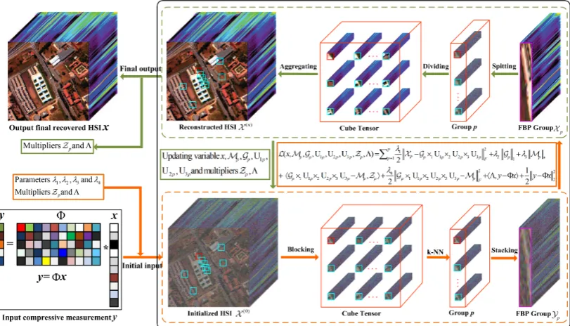
Figure 1.Flowchart of the proposed HSI-CSR algorithm, which consists of two steps: sensing and reconstruction. First, it acquires the compressive measurementyby a random sampling matrixΦ. Second, NTSRLR recovers an HSI from the measurementsy=Φx.
1. To the best of our knowledge, we are the first to exploit GCS and NSS to construct the nonlocal structure sparsity of HSI that is a faithfully structured sparsity representation form for HSI-CSR task.
2. For each cube that is formed by grouping nonlocal similar cubes, the tensor representation based on tensor sparse and low-rank approximation is introduced to encode the intrinsic spatial-spectral correlation.
3. The HSI-CSR task is treated as an optimization problem; we resort to alternative direction multiplier method (ADMM) [44] to solve it.
A preliminary version of this work has appeared in [45], which presents the basic approach. In [45], we established the nonlocal structured sparsity from the perspective of the tensor low-rank property, which adopts the two most commonly used tensor low-rank representation forms: tensor low-rank approximation and tensor low-rank decomposition. In this paper, we depict the nonlocal structured sparsity via the tensor low-rank approximation and sparse representation. Although the tensor low-rank decomposition and sparse representation are derived from the Tucker decomposition model, the former needs to preset the ranks along all dimension while the latter introduces anl1-based sparse term on core tensor. In practical application, the latter possesses the reliable capability to represent the high-dimension data by mitigating the tensor rank overfitting or underfitting. In addition, this paper adds: (1) the detailed background of HSI-CSR; (2) the theoretical analysis of NTSRLR; and (3) additional HSI-CSR experiments.
The remainder of this paper is organized as follows. Section2introduces the tensor notations and operations commonly used in this paper, and background of CS. In Section3, a novel algorithm for HSI-CSR based on the NTSRLR model is proposed. Section4demonstrates the results of extensive experiments and Section5draws the conclusion.
2. Notations and Background of HSI-CS
2.1. Notations
we introduce some necessary notations and preliminaries about tensor as follows. A tensor of order N, which corresponds to aN-dimensional data array, is denoted asX ∈RI1×···×In×···×IN. Elements
ofX are denoted asai1···in···iN, where 1≤ in ≤ In. Definitions of tensor terminologies in the paper
follow exactly the same description in [46]. DenotekX kF =hX,X i(∑i1i2,...,iN|ai1i2,...,iN|
2)1/2,kX k 1=
∑i1i2,...,iN
ai1i2,...,iN
andkX k0as theF-norm,l1norm andl0norm of a tensorX, respectively.kX k0≤ K means thatK is the number of non-zero entries ofX. It is convenient to unfold a tensor into a matrix during the algorithm. The “unfold" operation along the mode-non a tensorX is defined as unfoldn(X) := X(n) ∈ RIn×(I1×···×In−1In+1×···×IN), and its opposite operation “fold" is defined as
foldn(X(n)) := X. The Kronecker product of matricesA ∈ RI×J andB ∈ RK×L is a matrix of size
IK×JL, denoted by A⊗B. The multiplication of a tensorX with a matrixY ∈RIk×Jkon mode-kis denoted byX ×kY=Z, which also can be defined in terms of mode-kunfolding asZk=YXk.
Definition 1. (Tucker decomposition) [46]: The Tucker decomposition form of a tensorX is:
X =G×1U1×2· · · ×NUN (1)
whereG ∈RJ1×J2×···×JN is the core tensor and it reflects the interaction between components along different modes, andUn ∈RIn×Jn is the orthogonal factor matrix in each mode. Thus, we can achieve the k-unfolding
form of Tucker decomposition in Equation (1)
X(n)=UnG(n)(UN⊗ · · · ⊗Un+1⊗Un−1⊗ · · · ⊗U1) (2)
2.2. Background of HSI-CS
For a given HSIX ∈RW×H×S(W×Hspatial resolution andSspectral bands),x∈
RW HSdenotes
the vector form ofX. LetN =W HS, then the compressive measurementy ∈ RMcan be obtained from the following CS model:
y=Φx (3)
where Φ ∈ RM×N(M < N) denotes the compressive operator. The CS theory indicates that a sufficiently sparse signalx can be exactly reconstructed from only a few observationywhen the compressive operatorΦsatisfies the restricted isometry property (RIP) [11]. Under the RIP, the ill-posed recovery problem can be formulated into following form by pursuing the sparsest signalx, i.e.,
x =min
x kxk0, s.t.y=Φx (4)
wherek · k0denotesl0norm as a sparsity constraint. However, thel0norm minimization in Equation (4) is combinatorially NP-hard and unstable with the noise. For this reason, a feasible strategy is to replace nonconvexl0norm as a convexl1counterpart [15,47] as follows:
x =min
x kxk1, s.t.y=Φx (5)
The optimization for above l1-minimization CS problem can resort to iterative shrinkage algorithm [48] and Bregman Split algorithm [49].
the underlying structure in an HSI or handling the unwanted noise and artifacts in the CSR procedure. In our method, we try to cope with those problems by introducing more refined prior knowledge of an HSI to perfectly promote HSI-CSR performance.
3. The Proposed HSI-CSR via NTSRLR
Structured sparsity is of great importance to the HSI-CSR model that often reveals the rich self-repetitive structures over spatial domain and the highly correlated bands across the spectral domain. Several previous works exploiting nonlocal prior have indicated that the structured sparsity based on nonlocal self-similarity is fairly effective for image restoration [18,19]. However, the research works in HSI-CSR fields have not been documented. In this paper, we present a unified framework for HSI-CSR using the structured sparsity via nonlocal tensor sparse representation and low-rank approximation.
3.1. Non-Local Tensor Formula for Structure Sparsity
The proposed regularization model for structured sparsity consists of two steps: cube grouping for characterizing GCS and NSS and tensor formulation for sparsity enforcement.
3.1.1. Non-Local Structure Sparsity Analysis
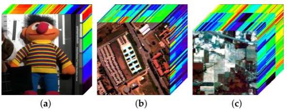
Concerning the GCS and NNS underlying an HSI, we provide an analysis for nonlocal tensor sparsity and low-rankness, as illustrated in Figure2. To begin with, for an initial third-order tensor HSIX ∈RW×H×S(e.g.,PaviaUdataset), we divide the HSI into a group of 3D full-band cubes (FBC) {Pi,j}1≤i≤W−w+1,1≤j≤H−h+1 ∈ Rw×h×S(w < W,h < H)with overlaps. For the exemplar cubePi,j of size 8×8× 60 located at spatial position(i,j)in Figure2a marked in red, we first search K-1 (here, we setK= 80) similar cubes by k-NN within a local window (e.g., 70×70), shown as k-NN clustering in Figure2b. Then, to avoid destroying the high spectral correlation, we unfold a series of 3D cubes into corresponding 2D matrices along the spectral modes (Figure2c), and obtain a new third-order tensorYp of size 64×80×60 by stacking a series of similar items (Figure2d), where p =1, . . .P, andPdenotes the group number. Such constructed third-order tensor simultaneously employ the spatial local sparsity (mode-1), the non-local similarity between cubes (mode-2) and strong spectral correlation (mode-3). The outcome of such arrangement maximizes the benefit from nonlocal tensor representation form. Next, we give a visual interpretation for the nonlocal tensor sparsity and low-rank property.
Figure 2.Nonlocal tensor sparsity and low-rank property analysis in HSI.
3.1.2. Non-Local Structure Sparsity Modeling
In Figure 2f, we can observe that the formed FBCs possess the low-rank property, and a tractable strategy is to use the mode-n rank(r1, . . . ,rn) to estimate tensor rank by Tucker decomposition [46]. For an Nth-order tensor X, the Tucker rank is defined as rank(X): = [rank(X(1)), rank(X(2)), . . . , rank(X(N))], where X(i) is the mode-i unfolding ofX [51]. Motivated by the practical applications that the nuclear norm is the convex envelope of the matrix rank within the unit ball of the spectral norm, further tensor nuclear norm,kX k∗ =∑n=N 1αn
X(n)
∗is defined
as weighting the unfolding matrix nuclear norm along each mode. Thus, we resort to the following relaxation form for eachXpto characterize the low-rank property based on GCS and NSS:
L(Xp) =
∑
3i αikXp(i)k∗ (6)wherekXp(i)k∗ =∑mink=1(m,n)σk(Xp(i))denotes the nuclear norm of matrixXp(i)of sizem×n.
In practice,{Yp}Pp=1may contain some noise, the dataYpcan be modeled as: Yp = Xp+Wp, whereXpandWpdenote the low-rank component and the noise component, respectively. Hence, we can estimate the low-rank tensorXpvia the following optimization problem:
Xp=min
Xp
L(Xp), s.t. Yp− Xp 2
F≤ε (7)
whereεis associated with the noise level. The model in Equation (7) is similar to the matrix cases
in [18], the difference primarily reflected in that we consider the combination with the correlations along local-nonlocal spatial modes and spectral mode, and measure the low-rankness of a third-order tensorXp by a weighted sum of the rank along each unfolding. Besides, considering the strong nonlocal spatial low-rankness along mode-2 than two other modes, we set a larger weight for mode-2 in our experiments.
under tensor sparse representation framework, thus each third-order tensorXpcan be approximated by following problem:
min
Gp,U1p,U2p,U3p
S(Gp), s.t.Xp=Gp×1U1p×2U2p×3U3p, UTipUip=I(i=1, 2, 3) (8)
where U1p, U2p, and U3pare factor matrices and S(Gp) is sparse constraint term, and we assume S(Gp) = Gp0as suggested in [42,43,52]. However, the optimization problem based onl0constraint
deduced by Equation (8) is non-convex, the research in [53,54] further relaxes thel0-based core sparsity tol1case as S(Gp) =
Gp
1. The convex optimization problem corresponding tol1 case can be
represented in Lagrangian form as following:
min
Gp,U1p,U2p,U3p
λ1 2
Xp− Gp×1U1p×2U2p×3U3p
2 F+λ2
Gp1, s.t. UTipUip= I(i=1, 2, 3) (9)
where λ1 and λ2 are the trade-off parameters. Essentially, all factor matrices are orthogonal dictionaries along local–nonlocal spatial modes and spectral mode. It can be seen that the tensor sparse representation model explores the GCS and NSS of HSIs in different dimensions by adaptive multi-dictionaries learning. Compared with the matrix sparse representation technique [19,20], the advantage of tensor modeling is that it not only characterizes the spatial-spectral correlation but also the correlation over nonlocal similar cubes in an HSI.
3.2. Proposed Model
Based on the previous analysis, we now derive the following model for solving the HSI-CSR problem:
min x,Gp,U1p,U2p,U3p
∑
P p=1
λ1 2
Xp− Gp×1U1p×2U2p×3U3p
2
F+λ2S(Gp) +λ3L(Xp),
s.t.y=Φx, UTipUip=I(i=1, 2, 3)
(10)
whereλ3is the regularization parameter. It is worth noting that the proposed model can fully exploit the underlying prior over spatial-spectral domain in an HSI, and thus is expected to have a strong ability to enhance HSI-CRS task.
3.3. Optimization Algorithm
For the proposed HSI-CSR model, we apply the ADMM [44], an effective strategy for solving large scale optimization problems, to solve Equation (10). Firstly, we replaceS(Gp)andL(Xp)with theGp1 and
Xp∗, respectively, and introduce Pauxiliary tensors {Mp}Pp=1 and equivalently reformulate Equation (10) as follows:
min
x,Mp,Gp,U1p,U2p,U3p
∑
P p=1
λ1 2
Xp− Gp×1U1p×2U2p×3U3p 2 F+λ2
Gp1+λ3Mp∗,
s.t.y=Φx,Mp=Gp×1U1p×2U2p×3U3p, UipTUip=I(i=1, 2, 3)
(11)
Then, its augmented Lagrangian function is:
L(Xp,Mp,Gp, U1p, U2p, U3p,Zp,Λ) =
∑
Pp=1λ1 2
Xp− Gp×1U1p×2U2p×3U3p
2 F+λ2
Gp1
+λ3
Mp∗+hGp×1U1p×2U2p×3U3p− Mp,Zpi+ λ4 2
Gp×1U1p×2U2p×3U3p− Mp 2 F
+hΛ,y−Φxi+1
2ky−Φxk 2 F
where {Zp}Pp=1 and Λ are the Lagrange multipliers, λ4 is the positive scalars. We shall break Equation (12) into five sub-problems and iteratively update each variable via fixing the other ones.
(a) U1p, U2p, U3pproblem:
min U1p,U2p,U3p
λ1 2
Xp− Gp×1U1p×2U2p×3U3p
2
F+hGp×1U1p×2U2p×3U3p− Mp,Zpi
+ λ4 2
Gp×1U1p×2U2p×3U3p− Mp 2 F, s.t. U
T
ipUip= I(i=1, 2, 3)
(13)
which is equivalent to the following sub-problem:
min U1p,U2p,U3p
∑
P p=1
G×1U1p×2U2p×3U3p− Op 2 F, s.t. U
T
ipUip=I(i=1, 2, 3) (14)
whereOp= λ1
Xp+∑3
i=1(λ4Mi−Zi)
λ1+3λ4 can be easily solved by the method as suggested in [53,54].
(b) Gpsub-problem:
min
Gp
λ1 2
Xp− Gp×1U1p×2U2p×3U3p 2
F+hGp×1U1p×2U2p×3U3p− Mp,Zpi
+λ4 2
Gp×1U1p×2U2p×3U3p− Mp 2 F+λ2
Gp
1
(15)
It can be rewritten as
min
Gp
1 2
Op− Gp×1U1p×2U2p×3U3p
2 F+λ2
Gp1 (16)
It can be solved by the Tensor-based Iterative Shrinkage Thresholding Algorithm (TISTA) in [53,54]. (c) Mpsub-problem:
min
Mp
λ3
Mp∗+hGp×1U1p×2U2p×3U3p− Mp,Zpi+λ4 2
Gp×1U1p×2U2p×3U3p− Mp 2 F,
(17)
It can be briefly reformulated as:
min
Mp
∑
3 i=1
λ3αi
λ4 Mp(i) ∗+ 1 2kBp+
Zp
λ4
− Mpk2F, (18)
whereBp=Gp×1U1p×2U2p×3U3p, its equivalent form is
min
Mp
∑
3 i=1
λ3αi
λ4 Mp(i) ∗+ 1
2kBp(i)+ Zp(i)
λ4
− Mp(i)k2F, (19)
As suggested in [51], its close-form solution is expressed as:
Mp(i)=foldi[Sαiλ3/λ4(Bp(i)+
Zp(i)
λ4
)], (20)
For a given matrix X, the singular value shrinkage operator Sτ(X) is defined as Sτ(X): = UXDτ(ΣX)VXT, and whereX=UXσXVXTis the SVD ofXandDτ(A) =sgn(Aij)(
Aij
(d) xsub-problem:
min
X
∑
P p=1
λ1 2
Xp− Gp×1U1p×2U2p×3U3p
2
F+hΛ,y−Φxi+ 1
2ky−Φxk 2
F, (21)
It is easy to observe that optimizingLwith respect toxcan be treated as solving the following linear system:
λ1x+Φ∗(Φx) =Φ∗(y−Λ) +λ1vec(X − G×1U1×2U2×3U3), (22)
whereG×1U1×2U2×3U3=∑Pp=1Gp×1U1p×2U2p×3U3p,vec(·)denotes the vectorization operator for a matrix or tensor, andΦ∗ indicates the adjoint ofΦ. Obviously, this linear system can be solved by well-known preconditioned conjugate gradient technique.
(e) Update the multipliers
(
Zp=Zp+ρλ4(Bp− Mp)
Λ=Λ+ρ(y−Φx) (23)
whereρis a parameter associated with the convergence rate at values of, e.g., [1.05–1.1]. The whole
optimization procedure for the proposed HSI-CSR model can be summarized as Algorithm 1, and we abbreviate the proposed method as NTSRLR.
Algorithm 1.HSI-CSR based NTSRLR.
Input:The compressive measurementsy, measurement operatorΦ, and the parameters of the algorithm. 1: Initialization:Initializing an HSIx(0)via a standard CSR method (e.g., DCT based CSR).
2: Forl=1 :Ldo
3: Extract the set of tensor{Xp}Pp=1fromx(0)via k-NN search the each exemplar cube; 4: Forp=1 :Pdo
5: Solve the problem (12) by ADMM;
6: Updating U1p, U2p, U3pby via Equation (14); 7: UpdatingGpvia Equation (16);
8: UpdatingMpvia Equation (20);
9: Updating the multipliersZpvia Equation (23); 10: End for
11: Updatingx(l)via Equation (22);
12: Updating the multiplierΛvia Equation (23); 13: End for
Output:CS Reconstructed HSIx(L).
4. Experimential Results and Analysis
4.1. Quantitative Metrics
To evaluate the HSI-CSR performances of all methods, five quantitative picture quality indices (PQIs) were employed in experiments. The first index is mean peak signal-to-noise ratio (MPSNR), which is defined as the average PSNR of all bands for HSI, e.g.
MPSNR(X, ˆX) = 1 S
∑
S
s=1PSNR(X
s, ˆXs), (24)
whereXs and ˆXs denotesth band images of ground truthX ∈
RW×H×S reconstructed HSI ˆX ∈ RW×H×S, respectively, and both of them are scaled to the range [0; 255].
The second index, mean structure similarity (MSSIM), was used to evaluate the similarity between the reconstructed HSI and the original HSI based on structural consistency, which is defined as average SSIM [59] of all bands for HSI,
MSSIM(X, ˆX) = 1 S
∑
S
s=1SSIM(X
s, ˆXs), (25)
The third index, mean feature similarity (MFSIM), emphasizes the perceptual consistency with the original image, which is defined as average FSIM [60] of all bands for HSI,
MFSIM(X, ˆX) = 1 S
∑
S
s=1FSIM(X
s, ˆXs), (26)
High values of these three measures MPSNR, MSSIM and MFSIM represent better reconstructed results.
The fourth index is the spectral angle mapper (SAM) [61], which calculates the average angle between spectrum vectors of the CS reconstructed HSI and the reference one across all spatial positions; its definition is as follows:
SAM(X, ˆX) =cos−1( x Txˆ √
xTx√xˆTxˆ), (27)
where x and ˆx denote vector form of the ground truthX reconstructed HSI ˆX, respectively.
The fifth index is the Erreur relative globale adimensionnelle desynth`ese (ERGAS) [62], which measures fidelity of the CS reconstructed HSI based on the weighted sum of MSE in each band, defined as follows
ERGAS(X, ˆX) =100
v u u
t
∑
S s=1
MSE(Xs, ˆXs)
µ2Xˆs , (28)
where MSE(Xs, ˆXs)is the mean square error betweenXsand ˆXs, andµ2 ˆ
Xs is the mean value of ˆXs.
Different from the former three PQI measures, smaller values of these two measures represent better reconstruction performances.
4.2. Experiments on Noiseless HSI Datasets
spatial-spectral resolutions and richer non-local similarity, which facilitates that the structured sparsity across spatial-spectral domains is employed in our HSI-CSR model. (2) These HSIs are benchmark testing datasets in HSI reconstruction, as presented in [21,22,24,25,40,42,43,45,50,53,54]. (3) We selected the dataset with classification label,Indian Pines, which helps to compare all methods in term of classification accuracy. For the experiment, we cropped a sub-region of 300×300 for all bands ofToy andPaviaU, as shown in Figure3. To validate the performance of proposed method, five different sampling rates (SR), namely 0.02, 0.05, 0.10, 0.15 and 0.20, were considered.
[image:11.595.152.448.195.310.2](a) (b) (c)
Figure 3.HSIs employed in the compressive sensing experiments: (a)Toy; (b)PaviaU; and (c)Indian Pines.
4.2.1. Visual Quality Evaluation
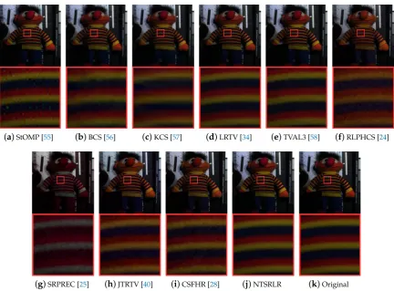
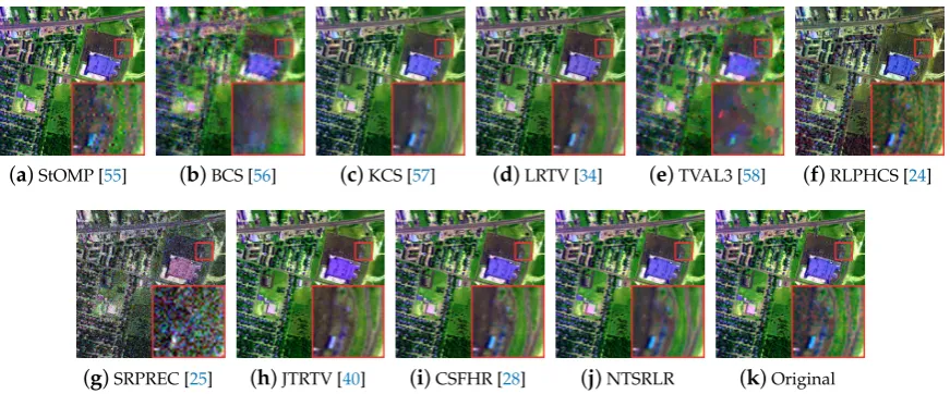
(a)StOMP [55] (b)BCS [56] (c)KCS [57] (d)LRTV [34] (e)TVAL3 [58] (f)RLPHCS [24]
[image:12.595.83.516.88.407.2](g)SRPREC [25] (h)JTRTV [40] (i)CSFHR [28] (j)NTSRLR (k)Original
Figure 4.Compressive sensing reconstructed results on pseudocolor images with bands (25,15, 5) of theToyimage from different methods under sampling rateρ= 0.20.
4.2.2. Quantitative Evaluation
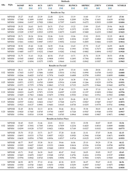
In Tables1and2, we provide the performance of all methods using MPSNR, MSSIM, MFSIM, SAM and ERGAS results, over all the spectral bands inToy,PaviaUandIndian Pines. We highlight the best results for each case in bold in the current and following tables. The proposed method outperforms the other approaches under all sampling rates and in particular the PQIs are better than the recent JTRTV. At sampling rateρ= 0.02, NTSRLR improves the MPSNR at least 10 dB more than JTRTV on
theToy, 1.3 dB better on thePaviaU, and 2.7 dB better on theIndian Pines. Forρ= 0.20, the average gain
(a)StOMP [55] (b)BCS [56] (c)KCS [57] (d)LRTV [34] (e)TVAL3 [58] (f)RLPHCS [24]
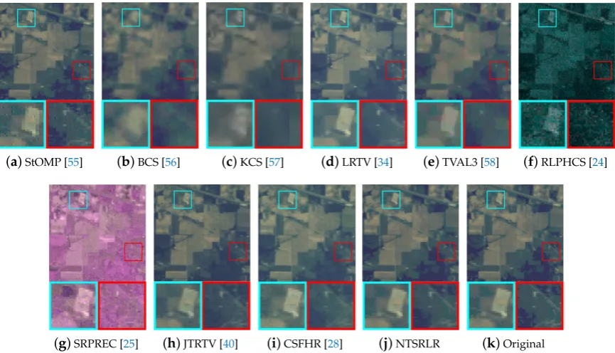
[image:13.595.84.517.91.403.2](g)SRPREC [25] (h)JTRTV [40] (i)CSFHR [28] (j)NTSRLR (k)Original
Figure 5.Compressive sensing reconstructed results on pseudocolor images with bands (55, 30, 5) of thePaviaUimage from different methods under sampling rateρ= 0.10.
(a)StOMP [55] (b)BCS [56] (c)KCS [57] (d)LRTV [34] (e)TVAL3 [58] (f)RLPHCS [24]
(g)SRPREC [25] (h)JTRTV [40] (i)CSFHR [28] (j)NTSRLR (k)Original
[image:13.595.83.516.452.700.2]The values of PSNR, SSIM and FSIM across all bands onIndian Pinesunder sampling rateρ= 0.10
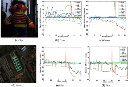
are presented in Figure7. The proposed method achieves the best PSNR, SSIM and FSIM values in most bands of the HSI, which also further validates the robustness of the proposed method over all spectral bands. To further illustrate the superiority of proposed NTSRLR on spectrum reconstruction, we chose four regions inToyandPaviaUdatasets shown Figure8a,d; the average reflectance differences were calculated between reconstructed spectra and original spectra across all bands. The curves of those average reflectance differences are plotted in Figure8b,c forToyand Figure8e,f forPaviaU. It is obvious that the reflectance difference between the reference and the reconstruction by NTSRLR is close to zero—much better than the other comparison methods.
[image:14.595.90.511.225.351.2](a)PSNR (b)SSIM (c)FSIM
Figure 7.PSNR, SSIM and FSIM values comparison of different methods for each band onIndian Pines
dataset under sampling rateρ= 0.20.
(a)Toy (b)Cyan (c)Green
(d)PaviaU (e)Red (f)Blue
Figure 8. Comparison of spectra difference onToyandPaviaUdatasets: (b,c) the spectra difference curves of different methods corresponding to the region marked by cyan and green rectangles of
[image:14.595.90.511.397.681.2]Table 1. MPSNRs, MSSIMs, and MFSIMs of different CSR methods on three selected HSIs under different sampling rates.
SRs PQIs
Methods
StOMP BCS KCS LRTV TVAL3 RLPHCS SRPREC JTRTV CSFHR NTSRLR [55] [56] [57] [34] [58] [24] [25] [40] [28]
Results onToy
0.02
MPSNR 25.27 18.45 23.39 22.08 22.91 13.19 14.40 17.19 25.87 27.81 MSSIM 0.7040 0.3499 0.6565 0.6651 0.6364 0.2089 0.2786 0.1601 0.6639 0.7322 MFSIM 0.8044 0.6937 0.7820 0.8061 0.7397 0.6651 0.6272 0.5033 0.8389 0.8484 0.05
MPSNR 29.35 24.63 26.93 26.51 27.63 13.22 13.89 22.65 29.96 34.22 MSSIM 0.8256 0.6672 0.7811 0.7873 0.7817 0.2372 0.1929 0.3374 0.7462 0.8930 MFSIM 0.9189 0.7837 0.8523 0.8783 0.8273 0.6493 0.5480 0.6233 0.8845 0.9423 0.10
MPSNR 29.71 28.24 29.94 32.06 31.81 13.06 15.92 29.93 32.35 40.12 MSSIM 0.8416 0.8072 0.8641 0.9233 0.8871 0.2034 0.1267 0.6860 0.8418 0.9640 MFSIM 0.9261 0.8563 0.8987 0.9517 0.9052 0.6163 0.4505 0.8466 0.9255 0.9814 0.15
MPSNR 30.90 29.40 31.88 34.99 33.46 13.69 27.79 31.47 34.99 44.52 MSSIM 0.8982 0.8429 0.9025 0.9427 0.9141 0.1993 0.7492 0.7673 0.8985 0.9848 MFSIM 0.9485 0.8777 0.9232 0.9669 0.9282 0.5642 0.9082 0.8894 0.9527 0.9928 0.20
MPSNR 31.75 31.63 33.26 40.54 37.65 13.71 25.74 33.39 38.53 47.86 MSSIM 0.9345 0.8845 0.9236 0.9808 0.9593 0.2495 0.7384 0.8504 0.9541 0.9925 MFSIM 0.9617 0.9094 0.9375 0.9876 0.9664 0.6182 0.8942 0.9307 0.9785 0.9965
Results onPaviaU
0.02
MPSNR 28.11 21.74 23.79 23.08 22.99 15.18 14.84 28.04 25.11 29.83 MSSIM 0.7603 0.4767 0.5486 0.6500 0.5014 0.1562 0.0990 0.6708 0.6923 0.8000 MFSIM 0.8246 0.6825 0.6743 0.7974 0.6429 0.6808 0.5758 0.8593 0.8095 0.8884 0.05
MPSNR 30.06 24.26 26.59 27.49 25.29 14.38 15.46 35.73 32.74 37.96 MSSIM 0.8571 0.5572 0.6783 0.8099 0.5914 0.1698 0.1266 0.9235 0.8756 0.9551 MFSIM 0.9371 0.7379 0.7854 0.8863 0.7132 0.7123 0.6379 0.9666 0.9442 0.9774 0.10
MPSNR 30.40 26.36 29.14 32.99 27.48 15.73 16.00 37.10 34.36 42.15 MSSIM 0.8223 0.6479 0.7871 0.9158 0.6907 0.1225 0.1157 0.9452 0.9062 0.9794 MFSIM 0.9409 0.7963 0.8606 0.9479 0.7894 0.5930 0.5461 0.9761 0.9583 0.9905 0.15
MPSNR 31.59 27.08 30.85 33.81 28.33 26.46 28.29 37.39 36.77 44.55 MSSIM 0.8707 0.6812 0.8422 0.9417 0.7268 0.6771 0.8567 0.9487 0.9417 0.9872 MFSIM 0.9523 0.8137 0.8981 0.9683 0.8165 0.8738 0.9255 0.9778 0.9741 0.9944 0.20
MPSNR 32.49 28.54 32.13 40.56 30.46 28.14 35.38 38.03 40.56 46.55 MSSIM 0.9020 0.7445 0.8745 0.9740 0.8057 0.7328 0.9547 0.9548 0.9705 0.9917 MFSIM 0.9594 0.8518 0.9198 0.9862 0.8745 0.8964 0.9800 0.9807 0.9871 0.9965
Results onIndian Pines
0.02
MPSNR 30.45 33.03 31.46 22.81 30.12 19.51 23.58 30.87 30.85 33.54 MSSIM 0.7487 0.7692 0.7385 0.4916 0.7839 0.2234 0.4025 0.8010 0.8089 0.8202 MFSIM 0.8299 0.8128 0.7337 0.8421 0.8026 0.7149 0.8327 0.8102 0.8500 0.8775 0.05
MPSNR 35.70 37.23 33.71 26.77 37.28 16.44 21.01 37.07 36.86 41.15 MSSIM 0.8693 0.8153 0.7763 0.8057 0.8221 0.0920 0.2944 0.9240 0.8671 0.9470 MFSIM 0.8639 0.8554 0.7983 0.8936 0.8517 0.4714 0.8125 0.9475 0.9210 0.9553 0.10
MPSNR 40.77 38.97 35.38 34.10 39.66 16.06 25.10 39.29 37.38 44.12 MSSIM 0.9395 0.8427 0.8165 0.9153 0.8606 0.0614 0.5336 0.9338 0.8798 0.9719 MFSIM 0.9420 0.8867 0.8491 0.9440 0.8919 0.3846 0.8317 0.9472 0.9439 0.9750 0.15
MPSNR 43.71 39.42 36.39 34.65 40.47 19.62 24.05 39.85 39.27 45.65 MSSIM 0.9465 0.8478 0.8417 0.9248 0.8743 0.4756 0.4416 0.9354 0.9197 0.9810 MFSIM 0.9794 0.8942 0.8743 0.9496 0.9056 0.7956 0.7804 0.9476 0.9569 0.9818 0.20
Table 2.SAM and ERGAS comparisons of different CSR methods on three selected HSIs under different sampling rates.
SRs PQIs
Methods
StOMP BCS KCS LRTV TVAL3 RLPHCS SRPREC JTRTV CSFHR NTSRLR
[55] [56] [57] [34] [58] [24] [25] [40] [28]
Results onToy
0.02 SAM 0.3040 0.6548 0.3062 0.5096 0.3888 0.9853 0.9707 0.6599 0.4014 0.2810 ERGAS 165.5 864.5 294.7 362.5 309.7 2411 2740 582.3 178.9 154.8
0.05 SAM 0.2500 0.2781 0.2351 0.3967 0.2886 0.9633 0.9210 0.6532 0.3401 0.2029 ERGAS 147.8 257.3 193.9 204.3 181.9 2064 2536 321.4 141.5 84.65
0.10 SAM 0.2318 0.1968 0.1894 0.2162 0.2080 0.6234 0.8382 0.4129 0.2750 0.1031 ERGAS 141.94 170.4 136.9 107.0 113.1 1273 1853 140.3 108.1 35.92
0.15 SAM 0.2629 0.1654 0.1635 0.1940 0.1828 0.4228 0.4562 0.3582 0.2151 0.0998 ERGAS 123.9 148.6 109.9 78.40 93.82 1262 1620 118.5 79.23 28.08
0.20 SAM 0.1123 0.1471 0.1478 0.1112 0.1294 0.3866 0.4250 0.2964 0.1599 0.0733 ERGAS 112.5 116.1 94.29 41.20 58.60 978 1305 95.77 53.85 20.86
Results onPaviaU
0.02 SAM 0.1819 0.2223 0.1931 0.1576 0.2460 0.9542 0.9950 0.1722 0.1248 0.1128 ERGAS 137.8 345.6 264.4 329.0 284.3 2537 3585 156.7 153.8 125.8
0.05 SAM 0.1542 0.1749 0.1512 0.1347 0.2021 0.8849 0.9646 0.0817 0.1019 0.0550 ERGAS 123.4 245.2 187.6 153.2 213.4 2079 2997 67.56 96.19 50.98
0.10 SAM 0.1447 0.1417 0.121 0.0862 0.1701 0.7069 0.8168 0.0725 0.0905 0.0389 ERGAS 118.7 188.0 138.7 90.35 165.2 1858 2425 58.58 80.19 32.53
0.15 SAM 0.1116 0.1326 0.1059 0.0708 0.1596 0.2914 0.2368 0.0708 0.0728 0.0315 ERGAS 103.6 173.3 113.96 77.17 149.8 1247 1921 56.68 61.15 24.90
0.20 SAM 0.0858 0.1178 0.0957 0.0462 0.1359 0.2407 0.0836 0.0674 0.0521 0.0260 ERGAS 93.40 146.2 98.66 38.73 117.7 1231 1427 52.63 41.26 19.74
Results onIndian Pines
0.02 SAM 0.1511 0.1622 0.1383 0.2774 0.1246 0.9166 0.9476 0.1075 0.1087 0.0821 ERGAS 143.2 161.8 138.6 759.7 126.5 1723 2297 129.7 198.7 116.0
0.05 SAM 0.1447 0.0830 0.1063 0.0832 0.0911 0.5668 0.8286 0.0553 0.0723 0.0382 ERGAS 89.48 88.69 119.2 233.2 87.85 1558 1988 64.84 152.6 49.62
0.10 SAM 0.0434 0.0728 0.0888 0.0587 0.0743 0.4821 0.6523 0.0515 0.0659 0.0282 ERGAS 38.77 74.77 96.91 43.08 68.53 1078 1323 58.37 127.4 35.96
0.15 SAM 0.0365 0.0714 0.0799 0.0498 0.0693 0.3914 0.4663 0.0505 0.0549 0.0229 ERGAS 34.98 72.32 86.24 37.45 62.99 917 1258 56.15 78.07 30.81
0.20 SAM 0.0295 0.0622 0.0741 0.0344 0.0586 0.2749 0.4590 0.0481 0.0553 0.0190 ERGAS 31.39 61.87 79.43 33.59 51.61 366 982 50.78 59.69 27.19
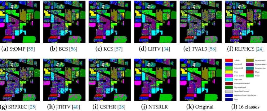
4.2.3. Classification Performance onIndian PinesDataset
The classification accuracy of the HSI with different algorithms was employed to further verify the effectiveness of the proposed method. Under the same circumstance, we chose the support vector machine (SVM) [63] and overall accuracy (OA) as the classifier and evaluation index, respectively. During the classification results with SVM algorithm, we used 16 ground-truth classes inIndian Pinesand 10% randomly generated training sets from each class to test the classification accuracy. The classification results with different HSI-CSR methods under sampling rateρ= 0.20 are revealed in
still show a continuous phenomenon, and the OA of NTSRLR is closer to the reference value. However, the classification results of other methods are more fragmentary in most regions of the image, with lower OA values.
(a)StOMP [55] (b)BCS [56] (c)KCS [57] (d)LRTV [34] (e)TVAL3 [58] (f)RLPHCS [24]
[image:17.595.85.516.141.320.2](g)SRPREC [25] (h)JTRTV [40] (i)CSFHR [28] (j)NTSRLR (k)Original (l)16 classes
Figure 9. Classification results for theIndian Pinesimage using SVM before and after CSR under sampling rateρ= 0.20.
Table 3.Classification performance comparison before and after CSR onIndian Pinesunder different sampling rates.
SRs StOMP BCS KCS LRTV TVAL3 RLPHCS SRPREC JTRTV CSFHR NTSRLR Original [55] [56] [57] [34] [58] [24] [25] [40] [28]
0.02 71.19% 50.64% 52.37% 60.96% 51.85% 29.61% 10.51% 20.03% 53.21% 73.69%
86.37% 0.05 75.70% 57.83% 56.18% 69.64% 57.83% 36.66% 13.32% 54.47% 59.17% 77.32%
0.10 76.32% 59.01% 62.01% 71.24% 60.92% 41.82% 14.62% 55.66% 62.98% 79.31% 0.15 78.41% 63.80% 65.80% 77.03% 62.70% 45.53% 45.53% 56.84% 65.24% 80.26% 0.20 80.28% 68.73% 70.73% 79.19% 65.73% 46.57% 57.83% 58.13% 67.70% 81.79%
4.3. Robustness for Noise Suppression during HSI-CSR
To further evaluate the effectiveness and robustness of proposed HSI-CSR method for noise suppression, we chose theUrbandataset (http://www.tec.army.mil/hypercube) contaminated by different degrees of mixture noise, which was with size of 307×307 and 4 m spatial resolution, and covers the wavelength in the range from 400 to 2400 nm by 10 nm spectral resolution. Under same competing methods, we removed 24 bands seriously affected by atmospheric attenuations and water absorptions, and finally reserved 186 bands for the dataset.
We present the pseudocolor image with bands (186, 131, 1), in which the input data is polluted by Gaussian noise and stripes, as shown in Figure10k. The CSR results produced by StOMP, BCS, CSFHR and TVAL3 could neither recover the original HSI nor perform the denoising task well. Instead, the methods RLPHCS and SRPREC amplified the noise. Although the methods KCS, LRTV and JTRTV could suppress the noise to some extent, they lost the edges and textural details when compared to NTSRLR.
[image:17.595.79.517.396.471.2](a)StOMP [55] (b)BCS [56] (c)KCS [57] (d)LRTV [34] (e)TVAL3 [58] (f)RLPHCS [24]
[image:18.595.83.519.90.271.2](g)SRPREC [25] (h)JTRTV [40] (i)CSFHR [28] (j)NTSRLR (k)Original
Figure 10.Compressive sensing reconstructed results on pseudocolor images with bands (186, 131, 1) of the noisyUrbanimage from different methods under sampling rateρ= 0.10.
(a)StOMP [55] (b)BCS [56] (c)KCS [57] (d)LRTV [34] (e)TVAL3 [58] (f)RLPHCS [24]
[image:18.595.91.516.314.469.2](g)SRPREC [25] (h)JTRTV [40] (i)CSFHR [28] (j)NTSRLR (k)Original
Figure 11.Horizontal mean profiles of compressive sensing reconstructed results on 1st band of real noisyUrbanHSI data from different methods under sampling rateρ= 0.10.
(a)StOMP [55] (b)BCS [56] (c)KCS [57] (d)LRTV [34] (e)TVAL3 [58] (f)RLPHCS [24]
(g)SRPREC [25] (h)JTRTV [40] (i)CSFHR [28] (j)NTSRLR (k)Original
Figure 12.Horizontal mean profiles of compressive sensing reconstructed results on 186th band of real noisyUrbanHSI data from different methods under sampling rateρ= 0.10.
[image:18.595.84.516.513.669.2]offer helpful remedy for its better image denoising. For tensor data, one can obtain the same results when unfolding a tensor into a matrix along certain mode, and the nonlocal tensor low-rank term of NTSRLR model can simultaneously provide complementary low-rank structures along all modes to promote the denoising performance of tensor data. Therefore, the noise of HSI can be suppressed to some extent. Besides, the research is [53,54] has demonstrated the effectiveness of tensor sparse models in multi-dimensional signals denoising, which verifies the positive impact of NTSRLR on noise suppression from the perspective of tensor sparse representation.
[image:19.595.83.515.282.511.2]Note that we removed all noisy bands and preserved only 171 bands for quantitative assessment. Table4presents MPSNR, MSSIM, MFSIM ERGAS and SAM of all methods under sampling rates 0.10, 0.15 and 0.20. It can be seen that our method not only recovered the structural and perceptual feature ofUrbandataset, but also preserved better spectral information.
Table 4. MPSNRs, MSSIMs, MFSIMs ERGAS and SAM of different CSR methods onUrbanwith different sampling rates.
SRs PQIs
Methods
StOMP BCS KCS LRTV TVAL3 RLPHCS SRPREC JTRTV CSFHR NTSRLR
[55] [56] [57] [34] [58] [24] [25] [40] [28]
0.10
MPSNR 19.63 16.95 23.63 24.76 17.79 22.04 15.13 27.74 26.76 30.88 MSSIM 0.6523 0.4147 0.8152 0.8705 0.4423 0.8155 0.4245 0.8959 0.8933 0.9471 MFSIM 0.8841 0.6918 0.8916 0.9277 0.6562 0.9088 0.7711 0.9561 0.9279 0.9746 ERGAS 280.2 380.4 184.2 159.6 346.3 261.6 480.9 111.5 109.8 76.89 SAM 0.2884 0.2157 0.1551 0.1197 0.2644 0.2737 0.4775 0.1196 0.1252 0.0682
0.15
MPSNR 20.61 17.45 25.78 26.40 18.48 24.16 20.94 27.94 28.27 33.51 MSSIM 0.7088 0.4546 0.8740 0.9134 0.4924 0.8442 0.8306 0.8992 0.9064 0.9662 MFSIM 0.8972 0.7138 0.9242 0.9575 0.6946 0.9284 0.9016 0.9580 0.9582 0.9845 ERGAS 250.4 359.7 145.4 122.9 320.0 202.4 296.3 108.9 91.23 56.89 SAM 0.2461 0.2076 0.1310 0.1024 0.2518 0.2202 0.2885 0.1180 0.1075 0.0564
0.20
MPSNR 20.93 18.72 27.37 33.26 20.35 25.99 25.24 28.40 30.11 35.62 MSSIM 0.7274 0.5509 0.9051 0.9664 0.6133 0.8583 0.9034 0.9040 0.9275 0.9762 MFSIM 0.9011 0.7645 0.9418 0.9840 0.7810 0.9459 0.9445 0.9608 0.9705 0.9896 ERGAS 241.4 310.8 122.3 59.45 259.0 165.8 183.7 103.1 67.60 44.66 SAM 0.2323 0.1879 0.1156 0.0592 0.2207 0.1831 0.1859 0.1149 0.0828 0.0481
4.4. Effectiveness Analysis of Single NTSR or NTLR Constraint
To further demonstrate the effectiveness of nonlocal tensor sparse representation and low-rank regularization in our model, we conducted two more experiments using thePaviaUdataset. The first experiment was to perform CSR without the nonlocal tensor low-rank regularization term, and the reconstructed HSI was achieved solely by nonlocal tensor sparse representation (NTSR). The second experiment was a reconstruction with the nonlocal tensor low-rank regularization method, but without NTSR, which is abbreviated as NTLR.
(a)MPSNR (b)MSSIM (c)SAM
Figure 13.MPSNR, MSSIM and SAM bars of different methods under sampling rates 0.05 to 0.20 with interval 0.05 onPaviaUdataset.
4.5. Computational Complexity Analysis
For an input HSIX ∈RW×H×S, the number of FBCs isP=O(W H), the size of each FBC group iswh×s×S, wheresis number of FBCs in each group. The computation cost seems not very small for quite largeP. However, CSR on thePFBCs can be processed in parallel, each with relatively small computational complexity. The computational complexity of the proposed algorithm that mainly lies in the update ofMp(i), Uip(i=1, 2, 3). Updating Uiprequires computing an SVD ofIi×Iimatrix, and updatingMp(i)requires computing an SVD ofIi×(∏j6=iIj)matrix. Relatively, the other variables Gp,xand multipliers updating will not consume lots of running time.
4.6. Convergence Analysis
Lastly, we have conducted experiments to show the convergence of our method using theToyand Indian Pinesdataset as examples under different sampling rates and different initializations. Figure14 plots the PSNRs versus iteration numbers for the tested HSIs when the sampling rates are at 0.10 for Toyand 0.15 forIndian Pines, when using initializationx=Φ∗yand DCT. As can be seen, the different initialization ways can provide quite close solutions, which indicates the performance of proposed algorithm is not sensitive to initialization. However, the two initialization ways possess different rates of convergence, and, by contrast, the initialization via DCT requires only a small number of iterations to get to the final PSNR. Therefore, we adopted the initialization strategy based on DCT to speed up our algorithm. Besides, the value of PSNR will become a constant when the algorithm converges. Thus, in the experiment, we set the maximum number of iterations for termination condition.
(a)ρ= 0.10 (b)ρ= 0.15
Figure 14.Verification of the convergence of the proposed method. Progression of the PSNRs for the
[image:20.595.156.447.557.694.2]4.7. Parameters Analysis
There are four parameters{λi}4i=1in the proposed model. Considering the different roles of nonlocal tensor sparseness and low-rankness terms, we conducted two more experiments onPaviaU dataset in Section4.4. The results of MPSNR, MSSIM and SAM demonstrate the nonlocal tensor low-rank regularization term plays a more important role in proposed model than nonlocal tensor sparse representation term. It implies that the nonlocal tensor low-rankness term should be assigned a greater weight to balance the two parts. Therefore, we setλ2=1 andλ3=10 in all our experiments. Correspondingly, we can regard the other two parts withλ1andλ4tradeoff as loyalty terms of the nonlocal tensor sparseness and low-rankness; it is reasonable to obtain a greater value forλ4, and we setλ1=0.02 andλ4=250, as suggested in [42].
Besides, the spatial size of cube and the number of non-local similar cubes are two key parameters. Some research [17,18,30,41] reports that the spatial size of cube and the number of non-local similar cubes are dependent on sampling rates. The higher the sampling rate is, the more detailed information of texture and structure the HSI loses. For this reason, the bigger spatial size and more non-local similar cubes are beneficial to provide extra knowledge to further promote the HSI reconstruction performance. Thus, according to the parameter setting principle in [17,18,30,41], we set spatial size to 6×6, 7×7, 8×8, 9×9 and 10×10 forρ= 0.20, 0.15, 0.10, 0.05 and 0.02, respectively; and the
corresponding number of non-local similar cubes are set to 50, 55, 60, 65 and 70.
5. Conclusions
In this paper, we propose a novel method for hyperspectral image compressed sensing reconstruction by non-local tensor sparse representation and low-rank regularization. The proposed method considers intrinsic structured sparsity, where the nonlocal similarity between spatial cubes and the global correlation across all bands are considered fully. Each cube group contains similar structures; its tensor-based sparsity and low-rank properties can be regarded as very valuable priors. Experimental results reveal that the proposed methods outperform the state-of-the-art methods in term of visual inspection, quantitative and classification accuracy assessment. The proposed method is also superior in noise suppression. We also conclude that it is advantageous to have integrated constraints using both non-local tensor sparse representation and low-rankness rather than using only one of them in our model.
Author Contributions: All authors contributed to the design of the methodology and the validation of experiments. J.X. wrote the paper. Y.Z., W.L. and J.C.-W.C. reviewed and revised the paper.
Funding:This work was supported by the National Natural Science Foundation of China (61371152 and 61771391), the Shenzhen Municipal Science and Technology Innovation Committee (JCYJ20170815162956949), and the Fund for Scientific Research in Flanders (FWO) project G037115N Data fusion for image analysis in remote sensing. Wenzhi Liao, a postdoctoral fellow of the Research Foundation Flanders (FWO-Vlaanderen), acknowledges its support.
Conflicts of Interest:The authors declare no conflict of interest.
References
1. Yang, J.; Zhao, Y.; Chan, J.C.-W. Learning and transferring deep joint spectral—Spatial features for hyperspectral classification.IEEE Trans. Geosci. Remote Sens.2017,55, 4729–4742. [CrossRef]
2. Yuan, Y.; Lin, J.; Wang, Q. Hyperspectral image classification via multitask joint sparse representation and stepwise MRF optimization.IEEE Trans. Cybern.2016,46, 2966–2977. [CrossRef]
3. Liu, Y.; Shi, Z.; Zhang, G.; Chen, Y.; Li, S.; Hong, Y.; Shi, T.; Wang, J.; Liu, Y. Application of Spectrally Derived Soil Type as Ancillary Data to Improve the Estimation of Soil Organic Carbon by Using the Chinese Soil Vis-NIR Spectral Library.Remote Sens.2018,10, 1747. [CrossRef]
5. Christophe, E.; Mailhes, C.; Duhamel, P. Hyperspectral image compression: Adapting spiht and ezw to anisotropic 3-d wavelet coding.IEEE Trans. Image Process.2008,17, 2334–2346. [CrossRef] [PubMed] 6. Töreyın B. U.; Yilmaz O.; Mert Y. M.; Türk F. Lossless hyperspectral image compression using wavelet
transform based spectral decorrelation. In Proceedings of the IEEE 7th International Conference on Recent Advances in Space Technologies (RAST), Istanbul, Turkey, 16–19 June 2015; pp. 251–254.
7. Wang, L.; Wu, J.; Jiao, L.; Shi, G. Lossy-to-lossless hyperspectral image compression based on multiplierless reversible integer TDLT/KLT.IEEE Geosci. Remote Sens. Lett.2009,6, 587–591. [CrossRef]
8. Mielikainen, J.; Toivanen, P. Clustered DPCM for the lossless compression of hyperspectral images.
IEEE Trans. Geosci. Remote Sens.2003,41, 2943–2946. [CrossRef]
9. Du, Q.; Fowler, J.E. Hyperspectral image compression using JPEG2000 and principal component analysis.
IEEE Geosci. Remote Sens. Lett.2007,4, 201–205. [CrossRef]
10. Du, Q.; Ly, N.; Fowler, J.E. An operational approach to PCA+JPEG2000 compression of hyperspectral imagery.
IEEE J. Sel. Top. Appl. Earth Observ. Remote Sens.2014,7, 2237–2245. [CrossRef]
11. Donoho, D.L. Compressed sensing.IEEE Trans. Inf. Theory2006,52, 1289–1306. [CrossRef]
12. Boufounos, D.; Liu, D.; Boufounos, P.T. A lecture on compressive sensing.IEEE Signal Process. Mag.2007,
24, 1–9.
13. Huang, J.; Zhang, T.; Metaxas, D. Learning with structured sparsity.J. Mach. Learn. Res.2011,12, 3371–3412. 14. Tan, M.; Tsang, I.W.; Wang, L. Matching pursuit LASSO part I: Sparse recovery over big dictionary.IEEE Trans.
Signal Process.2015,63, 727–741. [CrossRef]
15. Candes, E.J.; Wakin, M.B.; Boyd, S.P. Enhancing sparsity by reweightedl1minimization.J. Fourier Anal. Appl.
2008,14, 877–905. [CrossRef]
16. Chartrand, R.; Yin, W. Iterative Reweighted Algorithms for Compressive Sensing. In Proceedings of the IEEE International Conference on Acoust. Speech Signal Process, Las Vegas, NV, USA, 31 March–4 April 2008; pp. 3869–3872.
17. Dong, W.; Wu, X.; Shi, G. Sparsity fine tuning in wavelet domain with application to compressive image reconstruction.IEEE Trans. Image Process.2014,23, 5249–5262. [CrossRef]
18. Dong, W.; Shi, G.; Li, X.; Ma, Y.; Huang, F. Compressive sensing via nonlocal low-rank regularization.
IEEE Trans. Image Process.2014,23, 3618–3632. [CrossRef] [PubMed]
19. Dong, W.; Li, X.; Zhang, L.; Shi, G. Sparsity-based image denoising via dictionary learning and structural clustering. In Proceedings of the Computer Vision and Pattern Recognition (CVPR), Colorado Springs, CO, USA, 20–25 June 2011; pp. 457–464.
20. Mairal, J.; Bach, F.; Ponce, J.; Sapiro, G.; Zisserman, A. Non-local sparse models for image restoration. In Proceedings of the IEEE 12th International Conference on Computer Vision, Kyoto, Japan, 29 September–2 October 2009; pp. 2272–2279.
21. Zhang, L. Wei, W.; Zhang, Y.; Yan, H.; Li, F.; Tian, C. Locally similar sparsity-based hyperspectral compressive sensing using unmixing.IEEE Trans. Comput. Imaging2016,2, 86–100. [CrossRef]
22. Wang, L.; Feng, Y.; Gao, Y.; Wang, Z.; He, M. Compressed sensing reconstruction of hyperspectral images based on spectral unmixing. IEEE J. Sel. Topics Appl. Earth Observ. Remote Sens. 2018, 11, 1266–1284. [CrossRef]
23. Li, C.; Sun, T.; Kelly, K.F.; Zhang, Y. A compressive sensing and unmixing scheme for hyperspectral data processing.IEEE Trans. Image Process.,2012,21, 1200–1210.
24. Zhang, L.; Wei, W.; Tian, C.; Li, F.; Zhang, Y. Exploring structured sparsity by a reweighted laplace prior for hyperspectral compressive sensing.IEEE Trans. Image Process.2016,25, 4974–4988. [CrossRef]
25. Zhang, L.; Wei, W.; Zhang, Y.; Shen, C.; Hengel, A.V.D.; Shi, Q. Dictionary learning for promoting structured sparsity in hyperspectral compressive sensing. IEEE Trans. Geosci. Remote Sens. 2016, 54, 7223–7235. [CrossRef]
26. Fu, W.; Li, S.; Fang, L.; Benediktsson, J. A. Adaptive spectral—Spatial compression of hyperspectral image with sparse representation.IEEE Trans. Geosc. Remote Sens.2017,55, 671–682. [CrossRef]
27. Lin, X.; Liu, Y.; Wu, J.; Dai, Q. Spatial-spectral encoded compressive hyperspectral imaging.ACM Trans. Graphics (TOG)2014,33, 233. [CrossRef]
29. Meza, P.; Ortiz, I.; Vera, E.; Martinez, J. Compressive hyperspectral imaging recovery by spatial-spectral non-local means regularization.Opt. Express2018,26, 7043–7055. [CrossRef] [PubMed]
30. Wei, J.; Huang, Y.; Lu, K.; Wang, L. Nonlocal low-rank-based compressed sensing for remote sensing image reconstruction.IEEE Geosci. Remote Sens. Lett.2016,13, 1557–1561. [CrossRef]
31. Khan, Z.; Shafait, F.; Mian, A. Joint group sparse pca for compressed hyperspectral imaging.IEEE Trans. Image Process.2015,24, 4934–4942. [CrossRef] [PubMed]
32. Eason, D.T.; Andrews, M. Total variation regularization via continuation to recover compressed hyperspectral images.IEEE Trans. Image Process.2015,24, 284–293. [CrossRef] [PubMed]
33. Jia, Y.; Luo, Z. Weighted total variation iterative reconstruction for hyperspectral pushbroom compressive imaging.J. Image Process. Theory Appl.,2016,1, 6–10.
34. Golbabaee, M.; Vandergheynst, P. Joint trace/TV norm minimization: A new efficient approach for spectral compressive imaging. In Proceedings of the 19th IEEE International Conference on Image Processing (ICIP), Orlando, FL, USA, 30 September–3 October 2012; pp. 933–936.
35. Karami, A.; Yazdi, M.; Mercier, G. Compression of hyperspectral images using discerete wavelet transform and Tucker decomposition.IEEE J. Sel. Top. Appl. Earth Observ. Remote Sens.2012,5, 444–450. [CrossRef] 36. Wang, L.; Bai, J.; Wu, J.; Jeon, G. Hyperspectral image compression based on lapped transform and Tucker
decomposition.Signal Process. Image Commun.2015,36, 63–69. [CrossRef]
37. Zhang, L.; Zhang,L.; Tao, D.; Huang, X.; Du, B. Compression of hyperspectral remote sensing images by tensor approach.Neurocomputing2015,147, 358–363. [CrossRef]
38. Fang, L.; He, N.; Lin, H. CP tensor-based compression of hyperspectral images.J. Opt. Image Sci. Vis.2017,
34, 252. [CrossRef] [PubMed]
39. Yang, S.; Wang, M.; Li, P.; Jin, L.; Wu, B.; Jiao, L. Compressive hyperspectral imaging via sparse tensor and nonlinear compressed sensing.IEEE Trans. Geosci. Remote Sens.2015,53, 5943–5957. [CrossRef]
40. Wang, Y.; Lin, L.; Zhao, Q.; Yue, T.; Meng, D.; Leung, Y. Compressive sensing of hyperspectral images via joint tensor tucker decomposition and weighted total variation regularization.IEEE Geosci. Remote Sens. Lett.
2017,14, 2457–2461. [CrossRef]
41. Du, B.; Zhang, M.; Zhang, L.; Hu, R.; Tao, D. PLTD: Patch-based low-rank tensor decomposition for hyperspectral images.IEEE Trans. Multimed.2016,19, 67–79. [CrossRef]
42. Xie, Q.; Zhao, Q.; Meng, D.; Xu, Z.; Gu, S.; Zuo, W.; Zhang, L. Multispectral images denoising by intrinsic tensor sparsity regularization. In Proceedings of the IEEE Conference on Computer Vision and Pattern Recognition, Las Vegas, NV, USA, 27–30 June 2016; pp. 1692–1700.
43. Peng, Y.; Meng, D.; Xu, Z.; Gao, C.; Yang, Y.; Zhang, B. Decomposable nonlocal tensor dictionary learning for multispectral image denoising. In Proceedings of the IEEE Conference on Computer Vision and Pattern Recognition, Columbus, OH, USA, 23–28 June 2014; pp. 2949–2956.
44. Boyd, S.; Parikh, N.; Chu, E.; Peleato, B.; Eckstein, J. Distributed optimization and statistical learning via the alternating direction method of multipliers.Found. Trends Mach. Learn.2011,3, 1–122. [CrossRef]
45. Xue, J.; Zhao, Y.; Hao, J. Tensor non-local low-rank regularization for recovering compressed hyperspectral images. In Proceedings of the IEEE International Conference on Image Processing (ICIP), Beijing, China, 17–20 September 2017; pp. 3046–3050.
46. Kolda, T.G.; Bader, B.W. Tensor decompositions and applications.SIAM Rev.2009,51, 455–500. [CrossRef] 47. Schwab, H. For most large underdetermined systems of linear equations the minimall1solution is also the
sparsest solution.Commun. Pur Appl. Math.2006,59, 797–829.
48. Daubechies, I.; Defrise, M.; Mol, C.D. An iterative thresholding algorithm for linear inverse problems with a sparsity constraint.Commun. Pure Appl. Math.2004,57, 1413–1457. [CrossRef]
49. Zhang, X.; Burger, M.; Bresson, X.; Osher, S. Bregmanized nonlocal regularization for deconvolution and sparse reconstruction.SIAM J. Imag. Sci.2010,3, 253–276. [CrossRef]
50. Xue, J.; Zhao, Y.; Liao, W.; Kong, S.G. Joint spatial and spectral low-rank regularization for hyperspectral image denoising.IEEE Trans. Geosci. Remote Sens.2018,56, 1940–1958. [CrossRef]
51. Liu, J.; Musialski, P.; Wonka, P.; Ye, J. Tensor completion for estimating missing values in visual data.
IEEE Trans. Pattern Anal. Mach. Intell.,2013,35, 208–220. [CrossRef] [PubMed]
53. Qi, N.; Shi, Y.; Sun, X.; Yin, B. Tensor: Multi-dimensional tensor sparse representation. In Proceedings of the IEEE Conference on Computer Vision and Pattern Recognition, Las Vegas, NV, USA, 27–30 June 2016; pp. 5916–5925.
54. Qi, N.; Shi, Y.; Sun, X.; Wang, J.; Yin, B.; Gao, J. Multi-dimensional sparse models.IEEE Trans. Pattern Anal. Mach. Intell.2017,40, 163–178. [CrossRef]
55. Donoho, D.L.; Tsaig, Y.; Drori, I.; Starck, J.L. Sparse solution of underdetermined systems of linear equations by stagewise orthogonal matching pursuit.IEEE Trans. Inf. Theory2012,58, 1094–1121. [CrossRef]
56. Ji, S; Xue, Y.; Carin, L. Bayesian compressive sensing. IEEE Trans. Signal Process. 2008,56, 2346–2356. [CrossRef]
57. Duarte, M.F.; Baraniuk, R.G. Kronecker compressive sensing.IEEE Trans. Image Process.2012,21, 494–504. [CrossRef]
58. Li, C.; Yin, W.; Jiang, H.; Zhang, Y. An efficient augmented lagrangian method with applications to total variation minimization.Comput. Optim. Appl.2013,56, 507–530. [CrossRef]
59. Wang, Z.; Bovik, A.C.; Sheikh, H.R.; Simoncelli, E.P. Image quality assessment: From error visibility to structural similarity.IEEE Trans. Image Process.2004,13, 600–612. [CrossRef]
60. Zhang, L.; Zhang, L; Mou, X.; Zhang, D. Fsim: A feature similarity index for image quality assessment.
IEEE Trans. Image Process.2011,20, 2378–2386. [CrossRef]
61. Wald, L.Data Fusion: Definitions and Architectures: Fusion of Images of Different Spatial Resolutions. Presses des MINES: Paris, France, 2002.
62. Yuhas, R.H.; Boardman, J.W.; Goetz, A.F. Determination of semi-arid landscape endmembers and seasonal trends using convex geometry spectral unmixing techniques. InSummaries of the 4th Annual JPL Airborne Geoscience Workshop; NASA: Washington, DC, USA, 1993; Volume 4, pp. 205–208.
63. Melgani, F.; Bruzzone, L. Classification of hyperspectral remote sensing images with support vector machines,
IEEE Trans. Geosci. Remote Sens.2004,42, 1778–1790. [CrossRef]
64. Gu, S.; Xie, Q.; Meng, D.; Zuo, W.; Feng, X.; Zhang, L. Weighted nuclear norm minimization and its applications to low level vision.Int. J. Comput. Vis.2017,121, 183–208. [CrossRef]
c