Global Optimisation for Energy System

(1)

Global Optimisation for Energy

Systems

Ksenia Bestuzheva

October 2018

A thesis submitted for the degree of Doctor of Philosophy of The

Australian National University

(2)

Except where otherwise stated, this thesis is my own original work.

(3)

Abstract

The goal of global optimisation is to find globally optimal solutions, avoiding local optima and other stationary points. The aim of this thesis is to provide more efficient global optimisation tools for energy systems planning and operation. Due to the ongoing increasing of complex-ity and decentralisation of power systems, the use of advanced mathematical techniques that produce reliable solutions becomes necessary. The task of developing such methods is com-plicated by the fact that most energy-related problems are nonconvex due to the nonlinear Alternating Current Power Flow equations and the existence of discrete elements.

In some cases, the computational challenges arising from the presence of non-convexities can be tackled by relaxing the definition of convexity and identifying classes of problems that can be solved to global optimality by polynomial time algorithms. One such property is known as invexity and is defined by every stationary point of a problem being a global optimum. This thesis investigates how the relation between the objective function and the structure of the feasible set is connected to invexity and presents necessary conditions for invexity in the general case and necessary and sufficient conditions for problems with two degrees of freedom.

However, nonconvex problems often do not possess any provable convenient properties, and specialised methods are necessary for providing global optimality guarantees. A widely used technique is solving convex relaxations in order to find a bound on the optimal solution. Semidefinite Programming relaxations can provide good quality bounds, but they suffer from a lack of scalability. We tackle this issue by proposing an algorithm that combines decomposition and linearisation approaches.

In addition to continuous non-convexities, many problems in Energy Systems model dis-crete decisions and are expressed as mixed-integer nonlinear programs (MINLPs). The for-mulation of a MINLP is of significant importance since it affects the quality of dual bounds. In this thesis we investigate algebraic characterisations of on/off constraints and develop a strengthened version of the Quadratic Convex relaxation of the Optimal Transmission Switching problem.

(4)

Acknowledgements

First of all, I would like to thank my supervisory panel.

I am thankful to Dr. Hassan Hijazi for undertaking this journey with me, showing me interesting problems to work on and being an invaluable source of help on all aspects of the research process. Starting from the day when you welcomed me into the world of optimisation by placing a pile of papers in front of me (as I was sitting in the office wide-eyed, still confused by moving to another continent), continuing with the exciting discussions of the research lying ahead and sharing the hardships of model debugging and proof verifying, you have been a great mentor. You have been an example of scientific rigor and curiosity - the qualities that I will continue striving for in my further research career.

I am grateful to Prof. Sylvie Thiebaux for watching over the progress of my thesis and giving me valuable strategic advice. I greatly appreciate your guidance and support; despite you being a busy person, I have always felt that I could rely on you if I found myself in any difficult situation. As a passionate scientist and energetic and wise leader, you are an inspiration for me.

Many thanks also to Prof. Markus Hegland for being the mathematical sciences expert for this project, ready to help with any difficult proofs, and for inviting me to the group seminars where I could further extend my knowledge of mathematics. I enjoyed the atmosphere of genuine curiosity that you have created and encouraged at those seminars and will do my best to carry this attitude with me.

I gratefully acknowledge the funding provided by Data61, CSIRO for this work.

I would like to thank Dr. Carleton Coffrin for his contribution to the work on the Quadratic Convex relaxation of Optimal Transmission Switching, as well as others who were part of the optimisation team at that time for giving valuable feedback at the bi-annual presentations and creating a fun work environment (foosball!). I thank Dr. John Pye for letting me know about this Ph.D. program.

I express my deep appreciation to my mother for being with me through all the ups and downs of this journey, far in distance and time zones yet always close in heart; my grandmother for her loving and cheering presence on Skype; my grandfather for his support, and other family members. A special thanks to my friends both old and new for being great company, sharing passions, struggles or simply lunches and having conversations that were interesting, or heart-felt, or eye-opening, or funny or all those things at once.

(8)

(9)

Chapter 1

Introduction

The complexity of optimisation problems depends on the structure of the set of feasible so-lutions and the properties of the objective function. One crucial characteristic is convexity. Along with some mild nondegeneracy assumptions, convexity enables solving optimisation problems to global optimality or proving infeasibility with the use of polynomial time algo-rithms such as, for example, the widely used interior point methods.

However, many practical applications involve nonconvex constraints and objective func-tions, as well as discrete decisions. Among such application areas are energy systems, where the ongoing decentralisation and incorporation of renewable energy sources require solving challenging optimisation problems. Moreover, in energy systems the reliability of solutions is of critical importance in order to avoid system failures, and the requirements for compu-tational efficiency are often high due to large problem size and the need to solve problems repeatedly in real time. This creates the need for specialised methods that do not rely on convexity of the problem for providing globally optimal solutions.

Various techniques have been developed for this purpose. Inexact approaches such as approximations and heuristics might be able to find approximated global optima efficiently, but their applicability is limited when the reliability of the solutions is crucial. This has motivated research on techniques that provide provable optimality and feasibility guarantees. This thesis contributes to answering the following research question: given a nonconvex optimisation problem, how can we provide provable conclusions on its global optimum? In particular, how to show that the problem is infeasible or, given a feasible local optimal solution, prove its global optimality or evaluate the gap between this solution and the global optimum?

This work is focused on improving the performance of exact global optimisation methods as well as the quality of optimality guarantees provided. The goal is to extend the practical applicability of these methods to larger and more complex problems in energy systems.

(10)

relaxations of continuous problems and develops an algorithm that employs decomposition and linearisation in order to improve the scalability. Finally, we consider the case when the problem also involves discrete variables and on/off constraints, and the third part of the thesis presents a new formulation of quadratic on/off constraints and investigates ways of strengthening the Quadratic Convex relaxation [100] of the Optimal Transmission Switching problem in power systems.

Generalised Convexity

Under constraint qualifications [188] Karush-Kuhn-Tucker (KKT) conditions become both necessary and sufficient for global optimality in the case of convex problems [25]. Convexity, however, is not necessary in order for this property, known as KT-invexity, to hold and therefore can be generalised.

Since nonlinear solvers such as, for example, the interior-point solver Ipopt [187], provide polynomial time algorithms that do not in general find the global optimum but are guaranteed to converge to KKT points, KT-invexity enables their use for finding global optimal solutions. Moreover, identifying KT-invex subregions can improve the performance of spatial branch-and-bound algorithms.

Well known generalisations of convex functions include pseudo- and quasiconvex func-tions, and relaxations of the convexity property of optimisation problems have been proposed based on these notions. However, similarly to convexity, these conditions are not necessary for KT-invexity and there exist problems whose behaviour suggests KT-invexity, which are defined by nonquasi- and nonpseudoconvex functions. To gain more insight into the KT-invexity of such problems, one needs to consider the relations between the constraints and the objective function of the problem.

The conditions for KT-invexity that exist in the literature take these relations into account but, to the best of our knowledge, do not provide any clear procedure for identifying KT-invex problems. Therefore, the lack of algorithmically verifiable conditions still remains a major limitation of the invexity theory. We are addressing this by studying the behaviour of the objective function on the boundary of the feasible set and using it to identify classes of problems that are provably KT-invex. We define a new property which we call “boundary-invexity”, which ensures that certain structures that introduce multiple local minima are absent from the boundary of the feasible set. We prove that boundary-invexity is a necessary condition for KT-invexity in the generaln-dimensional case and a sufficient condition in the case of problems with two degrees of freedom.

(11)

KT-invexity of Optimal Power Flow The OPF problem has been proven to be NP-hard in the general case even for acyclic graphs [186, 124]. However, there is empirical evidence suggesting that OPF is KT-invex under some realistic assumptions on the parameter values and variable bounds, but a formal proof is necessary in order to guarantee global optimality of KKT points. As an example, we study invexity properties of a class of OPF problems with two degrees of freedom defined on networks that consist of two buses connected by one line. We show that under some realistic assumptions on the parameters, these problems are KT-invex.

Semidefinite Programming Relaxations for OPF

Many optimisation problems are not KT-invex or cannot be proven to be KT-invex using known methods, and efficient global optimisation algorithms are necessary in order to prove global optimality of their solutions. In such cases convex relaxations are widely used to evaluate the gap between a local optimal solution of a nonconvex problem and the global optimum.

Semidefinite programming (SDP) relaxations have been shown to yield tight bounds for the Optimal Power Flow (OPF) problem [122]. However, the scalability of the state of the art SDP solvers is limited.

Decomposition techniques such as constraint generation and exploiting sparsity of the graphs have been successfully applied to improve the efficiency of solution algorithms. Build-ing upon these results, we develop a linear cut generation algorithm which avoids addBuild-ing the computationally challenging SDP constraints to the model. First, we apply tree decomposi-tion to the sparsity pattern graph in order to obtain an equivalent formuladecomposi-tion of the SDP problem written in terms of smaller matrices. Then we investigate the impact of different lin-ear cuts on the slin-earch space, aiming to improve the reliability and efficiency of the approach. The notion of the “deepest valid cut” with respect to the Euclidean norm is introduced. In practice these cuts are obtainable by solving a projection subproblem. Using additional information about the problem such as which constraints tend to be active, we improve the SDP condition verification process, which allows us to detect more violated constraints and improve the gap yielded by our approach.

The resulting dynamic cut generation algorithm is applied to the Semidefinite Program-ming relaxation of the OPF problem and is shown to improve the robustness compared to standard SDP approaches.

(12)

bags. The proposed formulation is shown to be more computationally efficient than the standard sparse SDP formulation and yield the same bounds as the full SDP relaxation on medium-sized OPF test cases.

On/off Constraints and Convex Relaxations of Optimal

Transmission Switching

In Mixed-Integer Nonlinear Programs (MINLPs) the requirements on variables’ integrality are an additional source of non-convexity. For such problems the formulation plays a partic-ularly important role because it affects the quality of continuous relaxations which are used by branch and bound algorithms.

In this thesis we study constraints that are included into the model when the correspond-ing binary variable is equal to one and are ignored otherwise. Such constraints are referred to as on/off or disjunctive. In order to pass an on/off constraint to a MINLP solver, one has to find its algebraic formulation. Importantly, its continuous relaxation should be convex in order for the problem to be solvable to global optimality by efficient convex MINLP solvers which make use of the convexity of the continuous relaxation of the problem. Formulations that are written in the space of original variables and yield tight continuous relaxations typically lead to improved performance and thus are of interest.

We extend the perspective function based approach presented by Hijazi et al. [98] to non-monotone constraints by using the inverse of a function. Considering the feasible set of a two-dimensional quadratic on/off constraint as a union of two disjoint sets, we construct its algebraic formulation by finding the convex hull of those sets. The definition of a convex hull implies that such a formulation results in the tightest possible continuous relaxation. Moreover, our characterisation does not involve any additional variables. To avoid numerical issues arising from the nondifferentiability of perspective functions, we generate linear outer approximations of the convex hull.

New quadratic outer approximations of trigonometric functions are proposed, given that the function arguments have such bounds that ensure that the function is either convex or concave in the feasible set.

(13)

Main Contributions

Here we provide a brief summary of the main contributions of the thesis:

• An algorithmically verifiable necessary and sufficient condition for KT-invexity of prob-lems with two degrees of freedom;

• An algorithmically verifiable necessary condition for KT-invexity of problems with no restrictions on the number of degrees of freedom;

• A proof of sufficiency of global optimality on the boundary of the feasible set of a continuous nonconvex problem for global optimality in the interior;

• An algorithm for dynamic generation of linear Semidefinite Programming cuts with an application to the Optimal Power Flow problem;

• A compact characterisation of the convex hull of a two-dimensional quadratic on/off constraint;

• New quadratic outer approximations of trigonometric functions;

• A strengthened version of the Convex Quadratic relaxation of the Optimal Transmission Switching problem.

Structure of the Thesis

The structure of the thesis is as follows:

Chapter2provides a summary of basic optimisation concepts and reviews the application area of energy systems. It describes the Optimal Power Flow and Optimal Transmission Switching problems which motivated the theoretical research in this thesis and restates the formulations of their state of the art convex relaxations. The benchmarks that are used in the computational experiments are discussed.

In Chapter3we present the new conditions for KT-invexity and the necessity and suffi-ciency proofs. The connection between global optimality on the boundary and in the interior of the feasible set is established. The sufficient conditions are applied to prove KT-invexity of OPF problems with two degrees of freedom given mild assumptions on the variables’ bounds. Chapter4studies convex relaxations of nonconvex problems. We develop a dynamic cut generation algorithm based on decomposition and linearisation of SDP constraints and apply it to the Optimal Power Flow problem.

Chapter5continues the work on convex relaxations, focusing on mixed-integer programs. An algebraic formulation of a disjunctive constraint is proposed and new quadratic relax-ations of constraints with trigonometric functions are built. Together with some other tech-niques these results are used to tighten the Convex Quadratic relaxation of the Optimal Transmission Switching problem.

(14)

Notations and Basic Definitions

Throughout the thesis, we will use the following notation: BS boundary of a setS,

xi ith component of vector x,

f1

xi“ Bf

Bxi partial derivative off with respect toxi,

x¨y dot product of vectors xandy, xT _{transpose of vector}_x,

AB a segment between pointsAandB, 2N, 2N`1 the sets of even and odd numbers,

f1

´pxq, f`1pxq left and right derivatives off,

i imaginary unit,

<pxq real part of a complex numberx,

=pxq imaginary part of a complex numberx,

x˚ _{conjugate of a complex number}_x_,

|| ¨ || Frobenius norm of a matrix orl2_{-norm of a vector,} | ¨ | cardinality of a set orl1_{-norm of a scalar number,} convpSq convex hull of a setS.

Bold italic font will be used for constants and bold font will denote vectors.

Given a differentiable function f, Bf_Bp_uxq will denote the directional derivative off along vectoruwhich is defined as:

Bfpxq

Bu “ p∇fpxqq T

¨u.r192s

signpxqstands for the sign function:

signpxq “

$

’ ’ ’ &

’ ’ ’ %

(15)

Chapter 2

Background

This chapter provides background material that is relevant for the work presented in the subsequent chapters of this thesis. First, in Section2.1we restate some basic definitions and results from optimisation theory. Section2.2 concentrates on the nonconvex case and gives an overview of the methods that aim at providing global optimality guarantees.

Going on to the practical application, Section2.3presents the Alternating Current Op-timal Power Flow (AC-OPF) problem and discusses the optimisation techniques that have been applied to it. In Section2.4we review convex relaxations that have been proposed for the AC-OPF problem. Sections 2.5and2.6 consider a mixed-integer extension of AC-OPF known as Optimal Transmission Switching, present its formulation and convex relaxations.

The chapter is concluded by Section 2.7 which describes the benchmarks used for our computational experiments.

2.1 Optimisation Basics

In this section we recall some basic definitions and classical results in optimisation. Consider a constrained nonlinear optimisation problem in the following general form:

min fpxq

s.t.gipxq ď0, i“1, . . . , m, (N LPG)

hjpxq “0, j“1, . . . , k, xPRn,

wheref,gi, i“1 . . . , mand hj,j“1, . . . , kare twice differentiable functions. Some of the results discussed here can be extended to the nondifferentiable case, however, this is not the focus of this work. Let F denote the feasible set of (N LPG):

(16)

First, let us provide formal definitions of the solutions of optimisation problems. Finding a global optimum is most preferable:

Definition 2.1. [150] A point x˚ _P

Rn is a global minimiser for (N LPG) if x˚ P F and

fpxq ěfpx˚_q_for_x_P_F_.

However, in many cases most algorithms cannot guarantee global optimality and provably converge to a local optimum:

Definition 2.2. [150] A pointx˚_P

Rn is a local minimiser for (N LPG)ifx˚PF and there exists a neighbourhood Npx˚_q_{such that}_f_{pxq ě}_f_px˚_q_for_x_P_N_px˚_{q X}_F_.

If the inequality in the above definition is strict for all points in the neighbourhood except forx˚ _{itself, the minimiser is called strict:}

Definition 2.3. [150] A point x˚ _P

Rn is a strict local minimiser for (N LPG) if x˚ P F and there is a neighbourhoodNpx˚_q_{such that} _f_{pxq ą}_f_px˚_q_for_x_P_N_px˚_{q X}_F _z _x˚_.

First-order optimality conditions can be expressed in terms of constraint gradient vectors at a given point:

Definition 2.4. [109,117] A solutionx˚_{of problem}_{(N LPG)}_{is said to satisfy}

Karush-Kuhn-Tucker (KKT) conditions if there exist constants µi pi “1, . . . , mq and νj pj “ 1, . . . , kq, called Lagrange multipliers, such that

∇fpx˚

q “ ´ m

ÿ

i“1

µi∇gipx˚q ´ k

ÿ

j“1

νj∇hjpx˚q, (2.1)

gipx˚

q ď0, @i“1, . . . , m, (2.2)

hjpx˚q “0, @j“1, . . . , k, (2.3)

µiě0, @i“1, . . . , m, (2.4)

µigipxq “0, @i“1, . . . , m. (2.5) In the general nonconvex case, KKT conditions are necessary for a local optimum if constraint qualifications are satisfied. A widely used constraint qualification which we will utilise in this work is the linear independence constraint qualification:

Definition 2.5. [150] A pointx˚ _{is said to satisfy the linear independence constraint}

qual-ification (LICQ) if the set of active constraint gradients t∇gipx˚_q_{, i}_P_A_px˚_q_, _∇_h_jpx˚_q_{, j}_“

1, . . . , ku is linearly independent, where Apx˚_q _{be the set of indices of all active inequality}

constraints at point x˚_.

Further information on constraint qualifications can be found in the book by Nocedal and Wright [150].

(17)

Generally, first order conditions do not guarantee even local optimality. Second deriva-tives have to be considered in order to distinguish between local minima and other types of stationary points such as local maxima and saddle points. Second derivatives provide information about the local convexity/concavity of functions, and their role is to determine the behaviour of functions in the “undecided” feasible directions wwherewT_∇fpx˚_{q “}_0.

The set of directions that need to be considered in order to define second order conditions is known as a critical cone:

Definition 2.6. [150] Given a KKT point x˚ _{of problem} _{(N LPG)} _{and corresponding}

La-grange multiplier vectors µ, ν, a critical cone Cpx˚_{, µ, ν}_q _{is defined as a set of vectors} _w

such that:

$

’ ’ ’ &

’ ’ ’ %

p∇gipx˚_qqT

¨w“0 @iPApx˚_q_with_µ

ią0, p∇gipx˚_qqT

¨wď0 @iPApx˚_q_with_µ

i“0, p∇hjpx˚_qqT

¨w“0 @j“1, . . . , k,

whereApx˚_q_{is the set of indices of all active inequality constraints at point} _x˚_.

It can be observed that KKT conditions imply that wT_∇fpx˚_{q “} _{0 for all} _w _{in the}

critical cone. Therefore, critical cone contains undecided directions. Using this definition, we can write the second order conditions:

Theorem 2.1. [150](Second-order sufficient conditions) Letx˚ _{be a KKT point for problem}

(N LPG)with Lagrange multiplier vectorsµ,ν. Suppose that

wT_∇2_xLpx˚_{, µ, ν}_qw

ą0 @wPCpx˚_{, µ, ν}

q, w‰0,

where Lpx, µ, νq “fpxq ` m

ř

i“1

µigipxq ` k

ř

j“1

νjhjpxqis the Lagrangian function.

Thenx˚ _{is a strict local minimum in} _{(N LPG).}

Convex optimisation Iff,gi,i“1, . . . , mandhj,j “1, . . . , kare convex, (N LPG) is a convex optimisation problem.

For convex problems, KKT conditions (2.1)-(2.5) become both necessary and sufficient for a global optimum [25]. Other important results proven for convex problems include weak and, under constraint qualifications, strong duality, convergence and convergence rates of interior-point algorithms.

Since polynomial time algorithms exist that guarantee convergence to KKT points, convex problems are solvable to global optimality in polynomial time.

2.2 Global Optimisation Methods

(18)

2.2.1 Upper bounding methods

Local optimisation algorithms can be applied to nonconvex problems, but with significant limitations. In the case where certain generalised convexity properties such as, for example, pseudo- and quasi- convexity or invexity [131, 133], can be proven, some of these methods guarantee global optimality, but in the general case convergence even to a local optimum is not guaranteed. For example, such methods might converge to a saddle point or report local infeasibility. Since they cannot guarantee infeasibility of the whole problem, no informative conclusions can be made in the latter case.

Despite these issues, convex optimisation methods are widely used for evaluating an upper bound on the optimal solution of a nonconvex problem.

[image:18.612.220.432.281.448.2]

2.2.2 Convex relaxations

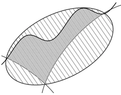
Figure 2.1: Example of a convex relaxation: the nonconvex set is shown in grey colour, the hatched region represents the relaxation

By definition, a convex relaxation of a nonconvex optimisation problem is a problem of optimising the same objective function over a convex set that includes the original feasible set. Therefore, the optimal objective function value of a relaxation is guaranteed to be less than or equal to the global optimum of the original problem [25] (or greater than or equal in the case of a maximisation problem). Such a value is called a lower bound. At the same time, a local optimum of the original (minimisation) problem is known to be greater than or equal to the global optimum and is referred to as an upper bound. Both values can be computed in polynomial time and can be used to evaluate how far from the global optimum the objective function value at a local solution is. If the lower bound equals the upper bound, the globally optimal value has been found. Moreover, if the relaxation is proven to be infeasible, so is the original problem.

(19)

2.2.3 Spatial branch and bound

The idea of spatial branch and bound algorithms [172, 180] is to systematically explore the feasible set by dividing it into smaller subregions. To divide the feasible region, a variable is chosen and its domain is separated into two parts, thus generating two subsets of the original set. This step is called branching. When exploring a subregion, local optimisation techniques, heuristics, convex relaxations and other methods are applied in order to obtain upper and lower bounds on the optimal solution. This process is known as bounding. By repeating these steps, upper and lower bounds are improved until a specified tolerance is reached.

Spatial branch and bound algorithms converge to the global optimum, although most often at a high computational cost.

2.2.4 Mixed-integer programming

In mixed-integer programming the integrality requirements on some variables present an additional computational challenge. Many methods that are commonly applied to solve such problems belong to the family of mixed-integer branch and bound methods [118, 50]. The idea is similar to that of spatial branch and bound with the following differences:

• the branching is done by choosing different values of the discrete variables,

• convex relaxations of nonconvex sets that are used in spatial branch and bound are replaced by continuous relaxations of mixed-integer sets.

A more detailed review of mixed-integer programming methods can be found in Section 5.2.

For solving nonconvex mixed-integer nonlinear programs, spatial and mixed-integer branch and bound can be combined in one algorithm.

2.3 The Optimal Power Flow Problem

(20)

2.3.1 Solution methods

AC-OPF is a challenging optimisation problem due to the nonconvex nature of physical laws governing the processes in the network. It has been proven to be NP-hard in the general case [186, 124]. Moreover, many OPF-based applications include discrete control elements and therefore need to be modelled as mixed-integer nonlinear programs. This has prompted extensive research on optimisation techniques tailored for OPF.

Local optimisation approaches include the adaptations of such classical nonlinear pro-gramming algorithms as gradient methods [53, 156], Newton-Raphson [36, 161], sequential linear and quadratic programming [175,176,27] and interior-point methods [83,183].

DC (direct current) approximations [162,163] have been widely used to linearise the OPF problem. These approximations model alternating current networks, and the name is derived from the observation that the linearised constraints resemble direct current power flow equa-tions. The DC model is computationally efficient and is a reasonably good approximation of AC power flows under normal operating conditions. However, it ignores reactive power and thus is not suitable for reactive power planning applications, and the key assumptions that ensure the accuracy of the model are often not satisfied [177]. A different linear approxima-tion that takes into account reactive power and voltage magnitudes was proposed by Coffrin and Van Hentenryck [44].

While approximations are useful for some applications, there is a need for methods that can provide provable optimality and feasibility guarantees. Recently there has been a lot of interest in convex relaxations of OPF since they can efficiently produce lower bounds on solutions. When combined with local optimisation techniques they can be used to eval-uate how far the objective function value at a local solution is from the global optimum. Convex relaxations are also used as part of spatial branch and bound algorithms [157,82]. Relaxations of the OPF problem are discussed in Section 2.4of this chapter.

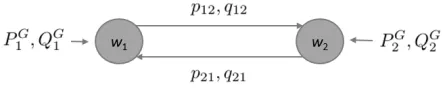
2.3.2 Formulation

Let us restate the formulation of the OPF problem. Consider an electrical network with the set of buses (nodes) and set of lines (arcs) denoted asN andE respectively. The following parameters and variables describe the physical characteristics of the network:

Parameters:

Yij“gij`ibij admittance of linepi, jq PE, where the real part is con-ductance and the imaginary part is susceptance, su

ij thermal limit of linepi, jq PE, Sd

i “pdi `iqid power demand at node i P N, where the real part is active power and the imaginary part is reactive power (demand is assumed to be constant),

(21)

Variables:

Sij “pij`iqij electric power along line pi, jq PE, consisting of active and reactive power,

Vi “vi=θi voltage at nodeiPNwith magnitudeviand phase angle

θi,

Wij “wRij`iwijI product of voltages at nodesiPN andjPN,

wi squared voltage magnitude at nodeiPN,

θij“θi´θj phase angle difference between nodesiPN andjPN,

Sig“p g i `iq

g

i power generation at nodeiPN, consisting of active and reactive power.

Upper indicesp¨ql andp¨qudenote lower and upper bounds on variables. The OPF problem in complex form is given by Model2.1:

Model 2.1: The Optimal Power Flow problem, complex form

variables for each pppi, jqqq PPPE:

Sij, Wij

variables for each iPPPN :

Vi, S g i

objective:

minÿ iPN

`

c2ip_<pSgiqq 2

`c1i_<pSigq `c0i

˘

(2.6a) subject to:

=Vr “0 (2.6b)

Wij “ViVj˚ @pi, jq PE (2.6c)

Sig´S d i “

ÿ

pi,jqPE

Sij`

ÿ

pj,iqPE

Sij @iPN (2.6d)

Sij “Yij˚Wii´Yij˚Wij @pi, jq PE (2.6e) |Sij| ďsuij @pi, jq,pj, iq PE (2.6f)

´tanpθu

ijq<pWijq ď=pWijq ďtanpθijuq<pWijq @pi, jq PE (2.6g)

<pS_iglq ď<pSigq ď<pS gu

i q @iPN (2.6h)

=pS_iglq ď=pSigq ď=pS gu

i q @iPN (2.6i)

pv_ilq2ď |Vi|2ď pv_iuq2 @iPN (2.6j)

(22)

constraints, OPF includes the operational constraints such as variable bounds and thermal limits ((2.6f)-(2.6j)) and the reference bus equation (2.6b). Unless specified otherwise, in all the models given here the lower and upper bounds on phase angle differencesθijare assumed to satisfy´π{2ăθl

ij ăθuij ăπ{2 and to be symmetrical (θlij“ ´θiju).

Model2.1 is often transformed into either the polar or rectangular real form. In both cases the apparent powerSijis replaced by the active and reactive powerspij,qij. The polar formulation is obtained by rewriting the complex terms by using the polar form of complex numbers and separating the equations that correspond to real and imaginary parts of the power flows:

Model 2.2: The Optimal Power Flow problem, polar form

pij, qij, θij P r´θuij, θ u ijs variables for each iPPPN :

viP rvil, vuis, θi

pgi P rp gl i , p

gu i s, q

g i P rq

gl i , q

gu i s objective:

minÿ iPN

`

c2ippgiq 2

`c1ip g i `c0i

˘

subject to:

θr “0 (2.7a)

θij “θi´θj @pi, jq PE (2.7b)

pgi ´p d i “

ÿ

pi,jqPE

pij`

ÿ

pj,iqPE

pij @iPN (2.7c)

qig´q d i “

ÿ

pi,jqPE

qij`

ÿ

pj,iqPE

qij @iPN (2.7d)

pij “gijv 2

i ´gijvivjcospθijq ´bijvivjsinpθijq @pi, jq PE (2.7e)

qij “ ´bijvi2`bijvivjcospθijq ´gijvivjsinpθijq @pi, jq PE (2.7f)

p2

ij`qij2 ďsuij @pi, jq PE (2.7g)

where equations (2.7c), (2.7d) are equivalent to (2.6d), constraints (2.7e), (2.7f) capture Ohm’s law (2.6e) and inequality (2.7g) enforces the thermal limits.

Alternatively, the voltages can be written using the rectangular form Vi “viR`iviI to obtain the rectangular formulation of OPF.

(23)

2.4 Relaxations of OPF

In this section we will review the convex relaxations of the OPF problem. The main idea behind these formulations is to substitute the nonlinear terms in the power flow equations by auxiliary variables and then impose convex constraints on these variables that capture certain aspects of the behaviour of the nonconvex expressions they represent.

2.4.1 Semidefinite programming relaxations

A semidefinite programming (SDP) constraint has the form:

X ľ0, (2.8)

requiring matrix X to be positive semidefinite (PSD). (2.8) describes a convex region. SDP constraints are often used for formulating convex relaxations of nonconvex continuous and combinatorial optimisation problems [144,78]. The SDP relaxation of OPF was introduced by Bai et al. [8]. Although computationally expensive, the SDP relaxation has the advantage of good solution quality. It has been proven to be exact in some special cases [122,173,195,

123]. The limitations of the SDP relaxation in terms of exactness were shown in a work by Lesieutre et al. [125], where a three-bus example with nonzero optimality gap was given.

The SDP formulation If we let

Wij“ViVj˚, (2.9)

then it can be observed that nonzeroVi,Vjsatisfying (2.9) exist if and only if the matrix

W “

$

&

%

Wii“wi @iPN,

Wij“wRij`iwijI @ pi, jq PNˆN,

is positive semidefinite and has rank 1. This allows us to eliminateV from the formulation by replacing (2.9) with:

W ľ0, rankpWq “1

and rewriting the power flow equations (2.6e) in terms of variableswi,wR

ij andwIij:

pij “gijwi´gijw R

ij´bijwijI @pi, jq PE,

qij“ ´bijwi`bijwRij´gijw I

ij @pi, jq PE.

(24)

angle differences are written as:

pvliq2ďwiď pviuq2, (2.10)

wijRtanpθ l ijq ďw

I ij ďw

R ijtanpθ

u

ijq. (2.11)

Bounds on the new variableswR ij andw

I

ij for allpi, jq PE are as follows: v_ilvl_jcospθu

ijq ďw R ijďv

u iv

u

j, (2.12)

´vuivjusinpθuijq ďwIijďvuivjusinpθuijq. (2.13) In the case when the linepi, jqdoes not exist (i.e. pi, jq P tNˆNuzE), the lower and upper bounds on the phase angle difference are instead defined by the sum of bounds (lower or upper, respectively) on the shortest path connecting nodesi andj. In practice, in order to avoid finding shortest paths between all nonadjacent nodes in the network, these are usually relaxed and replaced by the sum of bounds of all existing lines. Let Mu_,_Ml _{denote the} relaxed bound:

Mu“ ÿ

pi,jqPE

θ_iju, (2.14)

Ml“ ´Mu. (2.15)

Using this notation, we can now write the bounds on the remainingwR

ij,wIij variables:

wR ij ďv

u iv

u

j, (2.16)

$ ’ ’ ’ & ’ ’ ’ % wR ijěv

l iv

l jcospM

u

qifMuăπ{2, wR

ijěv u iv

u j cospM

u

qifπ{2ďMuăπ, wR

ijě ´v u iv

u

j ifπďM u_, (2.17) $ & % ´vu

ivuj sinpθijuq ďwijI ďviuvjusinpθuqifMuăπ{2, ´vu

ivuj ďwIij ďviuvuj ifπ{2ďMu.

(2.18)

The bounds calculated according to formulas (2.12)-(2.18) will be denoted as pwR ijql, pwR_ijqu,pw_ijIql andpw_ijIqu.

Obtaining the convex relaxation The rank 1 constraint captures all the non-convexity in OPF, therefore disregarding it results in a convex relaxation of the problem:

Model 2.3: The Semidefinite Programming relaxation of the OPF problem

(25)

pij, qij

variables for each pppi, jqqq PPPNˆˆˆN :

wR

ij P rpwRijql, pwRijqus, wijI P rpwijIql, pwijIqus variables for each iPPPN :

wiP rpvilq 2

, pv_iuq2s

pgi P rp gl i , p

gu i s, q

g i P rq

gl i , q

gu i s objective:

minÿ iPN

`

c2ippgiq 2

`c1ip g i `c0i

˘

subject to:

pgi ´p d i “

ÿ

pi,jqPE

pij`

ÿ

pj,iqPE

pij @iPN (2.19a)

qgi ´q d i “

ÿ

pi,jqPE

qij`

ÿ

pj,iqPE

qij @iPN (2.19b)

pij“gijwi´gijw R

ij´bijw I

ij @pi, jq PE (2.19c)

qij “ ´bijwi`bijwRij´gijwijI @pi, jq PE (2.19d)

p2

ij`qij2 ďsuij @pi, jq PE (2.19e)

wRijtanpθ l ijq ďw

I ijďw

R ijtanpθ

u

ijq @pi, jq PE (2.19f)

W ľ0 (2.19g)

The SDP formulation can be relaxed by disregarding all submatrices of size larger than two. The condition W ľ 0 is replaced with constraints requiring that principal minors of size 2 are nonnegative:

pwR

ijq2` pwijIq2ďwiwj @pi, jq PE.

Since the inequalities for minors of size 1 (wi ě 0) are dominated by squared voltage bounds, they are not included into the model.

This formulation is known as the Second Order Cone Programming (SOCP) relaxation. To the best of our knowledge, it was first proposed by Jabr [102] for radial networks. On such networks the above inequality is strictly equivalent to the full SDP constraint W ľ0 [173]. In other cases, although the bounds produced by the SOC relaxation are often weak, due to its computational efficiency this model can be used as a basis for dynamic constraint generation approaches [99, 112,138].

2.4.2 Quadratic Convex relaxation

Quadratic Convex (QC) relaxation was first proposed by Hijazi et al. [100]. As in the SDP relaxation, the wR

ij, w I

ij and wi variables represent the nonlinear nonconvex terms

(26)

these variables become linear. Each nonlinear term is treated as a composition of functions whose convex relaxations are formulated with the use of linear and quadratic constraints and combined in order to obtain the convex relaxation of the whole expression. This approach benefits from the typically small variable bounds in OPF problems, which can be further tightened by applying bound propagation [43].

The QC relaxation has been shown to yield better lower bounds than the SDP relaxation on some instances, which suggests that it captures those aspects of the original problem structure that the SDP formulation fails to account for [100,43].

To construct the Quadratic Convex formulation, new variables capturing the convex re-laxations of the underlying functions are introduced. Letcsij andsnij stand respectively for the convex relaxations of the cosine and sine functions ofθij. wij will denote the relaxation of the bilinear productvivj. Consistently with the notation used for describing the SDP re-laxation, variableswi,wR

ij andwIij represent the expressionsvi2,vivjcospθijqandvivjsinpθijq respectively. The following bounds on the new variables are enforced:

cospθu

ijq ďcsij ď1, (2.20)

´sinpθuijq ďsnij ďsinpθuijq, (2.21) v_ilvl_jďwij ďvuiv

u

j, (2.22)

pv_ilq2ďwi ď pvuiq

2_, _(2.23)

vilvljcospθuijq ďwRij ďvuivuj, (2.24) ´vliv

l jsinpθ

u ijq ďw

I ijďv

u iv

u j sinpθ

u

q. (2.25)

Trigonometric functions It is assumed that ´θl “ θu

ď π{2. Hijazi et al. [100] have proven that the following functions over- or underestimate trigonometric functions on r´θu_,_θu_s:

Proposition 2.1. [100] Let

p

cspθq “1´1´cospθ u

q pθu_q2 θ

2_.

Thencs_ppθq ěcospθq @θP r´θu_,_θu_s.

The above proposition provides a quadratic overestimator of cospθq. Since for θ P r´θu_,_θu

s the cosine function decreases as |θ| increases, it is easy to see that cospθuq ď cospθq @θP r´θu_,_θu_{s, therefore cospθ}u

ijqcan be used as the lower bound oncsij. Proposition 2.2. [100] Let

x

snpθq “cos

ˆ

θu 2

˙ ˆ

θ´θ u 2 ˙ `sin ˆ θu 2 ˙ , |

snpθq “cos

ˆ

θu 2

˙ ˆ

(27)

Thensn_|ďsinpθq ďsnxpθq @θP r´θ

u_,_θu_s.

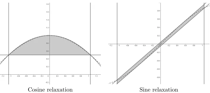
These results are used to construct valid convex relaxations of the cosine and sine func-tions shown in Figure2.2.

[image:27.612.151.505.152.309.2]

Cosine relaxation Sine relaxation

Figure 2.2: Convex relaxations of trigonometric terms

Quadratic terms The convex envelope for a quadratic function is written as:

wěv2,

wď pvl`vuqv´vuvl.

Multilinear terms The McCormick formulation [136] is applied to obtain convex relax-ations of the bilinear products. For example, given two variablesvi,vj and their lower and upper bounds, the McCormick relaxation of the productvivj has the form:

wij ěvilvj`vjlvi´vliv l j,

wij ěviuvj`vjuvi´viuvuj,

wij ďvilvj`vjuvi´vliv u j,

wij ďviuvj`vljvi´vuiv l j.

The set of numberswij satisfying the above inequalities will be denoted asM Cpvi, vjq. The relaxations of the trilinear terms are formulated by applying sequential McCormick relaxations. Thus the relaxation ofvivjcospθijqis written asM Cpwij, csijqand the relaxation ofvivjsinpθijqis written asM Cpwij, snijq.

(28)

Strengthening the model The QC relaxation can be strengthened by introducing in-equalities that are derived by considering line power losses:

pij`pji“rijlij, (2.26)

qij`qji“xijlij, (2.27)

lij ě

p2 ij`q2ij

wi

, (2.28)

and the bounds on the phase angle differences expressed in terms of thewR

ij,wIijvariables: tanpθl

ijqwRijďwijI ďtanpθijuqwijR.

The Quadratic Convex formulation The full formulation of the Quadratic Convex relaxation of OPF is given by Model 2.4.

Model 2.4: The Quadratic Convex relaxation of the OPF problem

variables for eachpppi, jqqq PPPE:

pij, qij

csij P rcospθijuq, 1s, snij P r´sinpθuijq, sinpθ u ijqs

wij P rvliv l j, v

u iv

u js, w

R ij P rv

l iv

l jcospθ

u ijq, v

u iv

u js

wI ij P r´v

l iv

l jsinpθ

u ijq, v

u iv u j sinpθ u qs

θijP r´θiju, θ u ijs

variables for eachiPPPN :

wiP rpvliq2, pviuq2s

pgi P rp gl i , p

gu i s, q

g i P rq

gl i , q

gu i s objective:

minÿ iPN

`

c2ippgiq 2

`c1ip g i `c0i

˘

subject to:

θr“0 (2.29a)

pgi ´p d i “

ÿ

pi,jqPE

pij`

ÿ

pj,iqPE

pij @iPN (2.29b)

qig´q d i “

ÿ

pi,jqPE

qij`

ÿ

pj,iqPE

qij @iPN (2.29c)

pij “gijwi´gijw R ij´bijw

I

ij @pi, jq PE (2.29d)

qij “ ´bijwi`bijwRij´gijw I

ij @pi, jq PE (2.29e)

´tanpθu

(29)

cospθu

ijq ďcsij ďcsppθi´θjq @pi, jq PE (2.29g) |

snpθi´θjq ďsnijďsnxpθi´θjq @pi, jq PE (2.29h)

v2

i ďwiď pvl`vuqv´vuvl @iPN (2.29i)

wij PM Cpvi, vjq @pi, jq PE (2.29j)

wijRPM Cpwij, csijq @pi, jq PE (2.29k)

wijI PM Cpwij, snijq @pi, jq PE (2.29l)

p2 ij`q

2 ijďs

u

ij @pi, jq PE (2.29m)

p2.26q ´ p2.28q (2.29n)

2.4.3 Linear relaxations

Linear relaxations generally lack the lower bound strength of the nonlinear formulations but have the advantage of fast performance. Moreover, when added to the model in a dynamic iterative process, linear constraints can produce tight bounds. Bienstock and Mu˜noz [22] proposed a linear formulation in a lifted space, deriving cuts that can be used to strengthen relaxations of OPF iteratively. The paper by Taylor and Hover [181] presents a relaxation based on network flow models. Coffrin et al. [41] continued this line of work and developed two relaxations. One is close to that introduced by Taylor and Hover [181], but enforces nonnegative line power losses (since power cannot be generated on lines). The other derived in a similar fashion to the copper plate approximations which are based on the balance of supply and demand throughout the network.

2.5 Optimal Transmission Switching

Line switching equipment allows to change the configuration of the network dynamically and thus enables significant savings [59,93,94,71,158]. Topology design for reducing generation costs was originally suggested by O’Neill et al. [152] and formalised by Fisher et al. [58], and is referred to as Optimal Transmissions Switching (OTS).

From a mathematical standpoint, OTS is a mixed-integer nonlinear nonconvex problem. A binary variablezij is associated with each linepi, jq PEand represents its state. Ifzij“0 (the line is switched off), then the power flow has to be set to zero since a deactivated line can transmit no power. This is achieved by modifying the Kirchhoff’s current law and thermal limit constraints. The phase angle differences are affected by line switching: their lower and upper bounds are replaced by constantsMl_and_Mu_{using the same reasoning as explained} in Subsection 2.4.1.

Model2.5shows the OTS problem in the polar form. Here the notation

xijP rxl1ij,x u1 ij;x

l0 ij,x

(30)

is used to specify on/off bounds on a variable and is equivalent to

$

&

%

xl1

ijďxijďxu1ij ifzij “1, xl0_ijďxijďxl0ij ifzij “0.

Model 2.5: The Optimal Transmission Switching problem, polar form

pij, qij zij P t0,1u

θij P r´θiju, θ u

ij; ´Mu, Mus variables for each iPPPN :

viP rvil, v u is, θi

pgi P rp gl i , p

gu i s, q

g i P rq

gl i , q

gu i s objective:

minÿ iPN

`

c2ippgiq 2

`c1ipgi `c0i

˘

(2.30a) subject to:

θr “0 (2.30b)

θij “θi´θj @pi, jq PE (2.30c)

pgi ´p d i “

ÿ

pi,jqPE

pijzij`

ÿ

pj,iqPE

pijzij @iPN (2.30d)

qig´q d i “

ÿ

pi,jqPE

qijzij`

ÿ

pj,iqPE

qijzij @iPN (2.30e)

pij “gijv 2

i ´gijvivjcospθijq ´bijvivjsinpθijq @pi, jq PE (2.30f)

qij “ ´bijvi2`bijvivjcospθijq ´gijvivjsinpθijq @pi, jq PE (2.30g)

p2 ij`q

2 ij ďs

u

ijzij @pi, jq PE (2.30h)

2.6 Relaxations of OTS

In addition to the same non-convexities as in the OPF problem, OTS contains binary vari-ables, which makes it even more challenging.

(31)

2.6.1 Quadratic Convex relaxation

To the best of our knowledge, the first convex relaxation proposed for the OTS problem is the QC relaxation [100].

Since OTS is an extension of OPF, the QC relaxation of the latter can be modified in order be applied to the former. Therefore we will not restate this formulation but will only describe the changes.

The main feature of OTS is that the power flowspij, qij along a line become zero when linepi, jqis switched off (i.e. whenzij “0). The modifications of the QC model must ensure that this condition is satisfied and preserve convexity of the continuous relaxation, since it is necessary so that the convex MINLP solvers would provide global optimality guarantees. Moreover, formulations that result in tight continuous relaxations are desirable since they tend to improve performance.

In order to achieve this, disjunctive constraints are introduced that affect the feasible re-gion only when the corresponding line is activated. To express these constraints algebraically, a well known method referred to as big-M relaxation [143] is used unless stated otherwise. For a general on/off constraint of the form gpxq ď 0 if z “ 1, the big-M formulation is written asgpxq ď p1´zqM, whereM is a constant that should be large enough so that the constraint becomes redundant atz“0 (hence the name “big-M”).

To ensure that variableswR

ij,wIij,csij,snij have zero values whenever the corresponding line is deactivated, on/off variable bounds are added to the model.

Cosine disjunction Given the upper bound onθdenoted asθu_{and the cardinality of the} set of arcs |E|, let CS0-1 _{denote the set of}

pcs, θ, zqthat satisfy the quadratic relaxation of the on/off constraint: cs“cospθqifz“1. Then pcs, θ, zq PCS0-1 if:

csďz´1´cospθ u

q pθu_q2 θ

2

` p1´zq1´cospθ u

q pθu_q2 p|E|pθ

u q2q.

Using this definition, the relaxation of cosine for each linepi, jq PE can be written as:

pcsij, θij, zijq PCS0-1ij .

Sine disjunction For the formulation of the on/off version of the sine relaxation, the results from [101] are used in the QC-OTS model [100]. For the disjunctive version of a linear constraint of the form aTx´bď0, where x“ px1, . . . , xnqT, a big-M-like algebraic formulation is given by:

n

ÿ

i“1

aixiďbz` p1´zq

¨

˚ ˝

n

ÿ

i“1 aiă0

aixl0` n

ÿ

i“1 aią0

aixu0

˛

‹

‚. (2.31)

LetSN0-1 _{denote the set of}

(32)

(2.31), we express it by the following inequalities:

sn´cospθu

1{2qθďzpsinpθ

u

1{2q ´cospθ

u

1{2qθ

u

1{2q ` p1´zqpcospθ

u

1{2q|E|θ

u `1q,

cospθu

1{2qθ´snďzpsinpθ

u

1{2q ´cospθ

u

1{2qθ

u

1{2q ` p1´zqpcospθ

u

1{2q|E|θ

u `1q, where θu

1{2“θ

u_{2.

The relaxation will require that for each linepi, jq PE the following holds:

psnij, θij, zijq PSNij0-1.

Current magnitude disjunction The current magnitude disjunction is expressed by a set of quadratic and linear constraints:

p2

ij`qij2 ď pvuq2lijzij @pi, jq PE

p2

ij`qij2 ďlijuwizij @pi, jq PE

lij“ pgij2 `b 2

ijqpwi`wj´2wijRq @pi, jq PE

Variable bounds The bounds for each variable where they differ in the ’off’ and ’on’ states are expressed using a general formula:

xl1_z_`_xl0_p1_´_z_{q ď}_x_ď_xu1_z_`_xu0_p1_´_z_q_,

wherexl1_,_xu1_{represent the lower and upper bounds when the corresponding binary variable} is equal to one and xl0_,_xu0 _{denote the bounds when the binary is equal to zero.}

Finally, McCormick relaxations (2.29j)-(2.29l) are rewritten with the use of a big-M for-mulation and thermal limit constraints are identical to constraints (2.30h) in the nonconvex OTS problem.

2.6.2 MISOCP relaxation

An approach based on the second order cone formulation has been proposed by Kocuk et al. [113]. In order to linearise the power flow equations, it uses the same variables wi, wR ij and wI

ij as the previously described formulations and introduces a new set of variables w j i which represent the on/off squared voltage at node i which is set to zero when linepi, jqis deactivated. These variables are characterised by the following constraints:

pwijRqlzij ďwijRď pwRijquzij, (2.32) pwijIq

l

zij ďwijI ď pw I ijq

u

zij, (2.33)

pv_ilq2zij ďw j i ď pv

u iq

2

(33)

wi´ pviuq 2_p1

´zijq ďwji, (2.35)

wji ďwi´ pvliq 2_p1

´zijq, (2.36)

pwR

ijq2` pwijIq2ďw j iw

i

j, (2.37)

where (2.32) and (2.33) represent the on/off bounds onwR ij andw

I

ij, constraints (2.34)-(2.36) are obtained by applying the McCormick relaxation to wji “wizij and inequality (2.37) is the second order cone constraint.

To strengthen the formulation, additional inequalities are applied as cuts based on con-straints that connect the phase angle difference with variables wR

ij andwijI: pθj´θi´atan2pwIij, w

R

ijqqzij“0,

as well as SDP conditions and a cycle-based OPF formulation that was proposed by the same authors [112].

2.7 Benchmarks

For the computational experiments we use version 17.08 of the Power Grid Lib (PGlib) benchmarks which can be found at https://github.com/power-grid-lib/pglib-opf.

The benchmark contains three sets of instances: standard instances with typical operating conditions and more challenging Active Power Increase (API) and Small Angle Difference (SAD) instances with network sizes ranging from 3 to 9241 nodes.

The API instances represent networks with congested operating conditions where the line thermal limits are binding. It has been observed that optimal network topology depends on the loading scenarios [59], and considering networks where power flow congestion occurs leads to interesting OTS cases. The API instances are obtained by removing bounds on generator power output and solving active power increase problems which increase active loads until line thermal capacities become binding. The values of power generation and loads then define the new test cases [39].

Small phase angle differences provide better power system stability and impact optimi-sation approaches [44, 45, 100]. The SAD instances are constructed by solving small angle difference problems, where the objective is to find the minimum phase angle difference bound that, when applied to all lines in the network, does not result in infeasibility. Reduced angle differences provide guarantees in terms of power systems stability and impact optimization approaches, resulting in more challenging test cases with larger optimality gaps.

(34)

Chapter 3

Conditions for KT-Invexity

3.1 Introduction

In this chapter we focus on a special class of generalised convex problems called KT-invex problems, for which every point satisfying KKT conditions (2.1)-(2.5) is the global optimum. The polynomial time algorithms that converge to a local optimum in the general case will always find the global optimum for invex problems. This is often the case for OPF problems with realistic parameters. However, KT-invexity needs to be proven theoretically in order to guarantee global optimality for such problems.

The main idea behind generalised convexity is to identify the key features of convex func-tions and problems from a global optimisation point of view. As we will discuss in more detail below, the most popular approach has been to start with the well known characterisation of convex functions: given a convex setCPRn and a functionf : Rn ÑR,

f is convex onC ô fpxq ´fpyq ě px´yqT ¨∇fpyq @x,yPC, (3.1) and propose different relaxations of this condition.

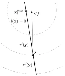
This work introduces a new way of looking at KT-invexity of optimisation problems. We notice that for maximisation problems with a concave objective, the properties of the boundary of the feasible set define whether the problem is KT-invex. More specifically, it is the behaviour of the objective function on the boundary that is key to determining KT-invexity. There exists a subset of “problematic” points whose existence leads to multiple local optima. These points can be found by studying different sections of the boundary corresponding to individual constraints.

This chapter defines a property, which we refer to as boundary-invexity, that is requir-ing that a problem does not have any “problematic” points. We prove its necessity for KT-invexity in the case of n-dimensional problems and establish the equivalence between boundary-invexity and KT-invexity for problems with two degrees of freedom.

This chapter is organised as follows.

(35)

and restates some key results on KT-invexity and its variations. In Section3.3we introduce the notion of boundary-invexity, prove its necessity for KT-invexity and study its connection to the local optimality of KKT points. Here we also establish the connection between global optimality on the boundary and in the interior.

After proving these results, we proceed to laying the technical foundation for the more challenging proof of sufficiency of boundary-invexity for KT-invexity of problems with two degrees of freedom. Section3.4proves some properties of a pseudo-scalar product of vectors. In Section3.5we define a parametrisation of the boundary curve. In Section3.6we study the behaviour of concave functions on a line and present some results on boundary-optimality.

Section 3.7presents the main theorem establishing the sufficiency of boundary-invexity for two-dimensional problems. Boundary-invexity of the Optimal Power Flow problem is investigated in Section3.8. Finally, Section3.9concludes the chapter and discusses ideas for future work.

3.2 Generalised Convexity

3.2.1 Early generalisations

Many practical applications involve non-convexities, and therefore the results proven for convex problems cannot be directly applied to them. However, convexity is not necessary for some convenient properties of optimisation problems to hold.

This has motivated research on finding various relaxations of convexity that preserve cer-tain key characteristics of convex problems. Among the first generalised convexity concepts were pseudo- and quasi-convexity proposed by Mangasarian [131]. These definitions were obtained by relaxing condition (3.1) by replacing the inequality with an implication. One such relaxation leads to the definition of pseudo-convex functions:

f is pseudo-convex onC ô

px´yqT ¨∇fpyq ě0 ñ fpxq ěfpyq @x,yPC,

and another results in the definition of quasi-convex functions:

f is quasi-convex onC ô

fpxq ďfpyq ñ px´yqT ¨_∇fpyq ď0 @x,yPC.

(36)

3.2.2 Invexity

It can be noticed that the main proofs of the properties of problems involving convex and generalised convex functions do not explicitly depend on the linear term in the definition, thus allowing for further relaxations. Therefore another direction of generalisation is based on modifying the expressions in the definition of convexity (3.1) ([5,6,19,33]). In invex functions introduced by Hanson [91] the linear term is replaced by an arbitrary vector functionη: Definition 3.1. A functionf : Rn Ñ Ris called invex onC if

fpxq ´fpyq ěηpx,yq ¨_∇fpyq @x,yPC

for some arbitrary vector function η: CˆC ÑRn.

The term “invex” was introduced by Craven [49], meaning “invariant convex”, since an invex function can be created by taking a composition of a differential injective coordinate transformation and a convex function. Ben-Israel and Mond [18] proved that a function is invex if and only if its every stationary point is a global minimum.

In constrained optimisation, invexity of functions has a connection to a property known as KT-invexity. Consider the optimisation problem:

maxfpxq

s.t. gipxq ď0@i“1, . . . , m, (NLP) xPRn,

where functions f and gi pi“1, . . . , mqare twice continuously differentiable and f is con-cave. The results in this chapter can be extended to problems with pseudoconcave objective functions since only convexity of the superlevel sets of f and the signs offpxq ´fpyqand p∇fpyqqT¨ px´yq,x,yPRnare used in the proofs. LetF denote the feasible set of (NLP).

Definition 3.2. [133] An optimisation problem is said to be Kuhn-Tucker invex (KT-invex) if every KKT point is a global optimiser.

Hanson [91] proved that KT-invexity holds if all functions in a problem are invex with respect to the same vector function η. Craven [47] proposed an equivalent characterisation of the latter property by requiring that a vector function that depends on all functions in the problem and some vector function η is nonnegative. In the same work, based on this characterisation, K-invex vector functions were defined by relaxing the non-negativity condition and requiring that the values of the vector function belong to a cone. Another characterisation was introduced by Martin [133] by relaxing the invexity condition on the constraints and enforcing it only on the boundary of the feasible set. This condition has been proved to be necessary and sufficient for KT-invexity.

Theorem 3.1. [133] (NLP)is KT-invex if and only if there exists a functionη:RnˆRn Ñ

(37)

x,yPF ñ

$

&

%

fpxq ´fpyq ´ηpx,yq ¨_∇fpyq ě0

gipyq “0ñηpx,yq ¨_∇gipyq ě0 @i“1, . . . , m.

Practical applicability of this condition is limited by the need to find anηthat will satisfy the inequalities for the objective function as well as all constraints.

Alternative formulations of the invexity conditions have been suggested in an attempt to tackle this difficulty. A characterisation that does not require finding a common functionη

was proposed by Craven [48]. Consider a twice differentiable vector functionF : RnÑRm.

Observe that a vector function being invex is equivalent to all its components being invex with respect to the sameη, and these properties can be used interchangeably. Craven gives the following condition for the invexity ofF:

Theorem 3.2. [48]F is invex atx˚ _{if and only if}

p0‰αPRm`, α

T

¨∇Fpx˚

q “0q ñαT ¨F#px´x˚_,_x˚

q ě0, where F#_px

´x˚_,_x˚_q_{represents the higher-order terms in the Taylor expansion of}_F_:

F#px´x˚_,_x˚

q “Fpxq ´Fpx˚

q ´ p∇Fpx˚

qqT¨ px´x˚

q.

However, the evaluation ofF#_px

´x˚_,_x˚_q_{is not straightforward. Another}

characterisa-tion has been derived [48] based on Theorem3.2:

Theorem 3.3. [48] Consider the Wolfe dual for (NLP):

max`

´fpuq `vT ¨Gpuq˘ s.t.vě0, ´∇fpuq `vT ¨∇Gpuq “0,

where G: RnÑRm is a vector comprised of all constraint functionsgi.

For each feasible pointpu,vq, assume that _∇Gpuq has full rank,_∇fpuq ‰0, and ´fpzq `vT ¨Gpzq ě ´fpuq `vT ¨Gpuq @z. (3.2) Thenpf, Gqis invex atpu,vq.

This condition is difficult to verify because (3.2) needs to be checked for every feasible point pu,vq. Moreover, identifying whether uis the global minimum of´fpzq `vT

¨Gpzq over allzis NP-hard since it is a nonconvex problem.

A different approach has been introduced by Mart´ınez-Legaz [135] by considering linear combinations of functions:

Theorem 3.4. [135] A differentiable vector function F : Rn ÑRm is invex if and only if

the function m

ř

i“1

λifi is invex for all pλ1, . . . , λmq P Rm, where functions fi : Rn Ñ R for

(38)

However, checking the invexity of all linear combinations is a difficult problem.

To the best of our knowledge, the lack of algorithmically verifiable conditions still remains a major limitation of the invexity theory which we are starting to address in this chapter.

3.3 New Conditions for Kuhn-Tucker Invexity

Let us emphasise that checking local optimality is NP-hard in general:

Theorem 3.5. [155] The problem of checking local optimality for a feasible solution of (NLP)is NP-hard.

In this work, we try to investigate necessary and sufficient conditions that allow us to circumvent the negative result presented in Theorem3.5by identifying problems where KKT points are provably global optimisers.

3.3.1 Weak boundary-invexity

For each nonconvex constraintgipxq ď0 define the problem:

min fpxq (NLPi)

s.t. gipxq “0.

The objective in (NLPi) is opposite to that in (NLP), for example, if a function is to be maximised in (NLP), then (NLPi) should minimise the same function.

First let us restate the definition of a strict local minimiser: Definition 3.3. [150] A point x˚_P

Rn is a strict local minimiser for (NLPi)if gipx˚q “0 and there is a neighbourhoodNpx˚

qsuch thatfpxq ąfpx˚

qforxPNpx˚

q zx˚

| gipxq “0. Now we can define a new property that we refer to as weak boundary-invexity:

Definition 3.4. (Weak boundary-invexity) Problem (NLP)is weakly boundary-invex if for every ithat corresponds to a nonconvex constraint either the problem (NLPi)does not have a finite global optimal solution x˚ _{or at least one of the following holds:}

1. x˚ _{is infeasible for} _(NLP),

2. x˚ _{is not a strict minimiser for} _(NLPi),

3. the Lagrange multiplier forx˚ _in _(NLPi)_{is nonnegative,}

4. there exist constraints gjpxq ď0, j‰iin (NLP) that are active atx˚_.

Global Optimisation for Energy System