On the use of probabilistic model-checking for the verification of prognostics applications

On the use of Probabilistic Model-Checking for the

Verification of Prognostics Applications

Jose Ignacio Aizpurua and Victoria M. Catterson,

Senior Member, IEEE

University of Strathclyde Glasgow, United Kingdom

[email protected], [email protected]

Abstract—Prognostics aims to improve asset availability

through intelligent maintenance actions. Up-to-date remaining useful life predictions enable the optimization of maintenance planning. Verification of prognostics techniques aims to analyze if the prognostics application meets the design requirements. Online prognostics applications depend on the data-gathering hardware architecture to perform correct prognostics predictions. Accordingly, when verifying prognostics requirements compliance, it is necessary to include the effect of hardware failures on prognostics predictions. In this paper we investigate the use of formal verification techniques for the integrated verification of prognostics applications including hardware and software components. Focusing on the probabilistic model-checking approach, a case study from the power industry shows the validity of the proposed framework.

Keywords—prognostics; verification; metrics; model checking

I. INTRODUCTION

Prognostics is an emerging field focused on the estimation of the Remaining Useful Life (RUL) of assets. Based on the available data and/or degradation equations, prognostics models predict the RUL of assets deployed in some specific conditions [1]. Prognostics predictions enable the optimization of maintenance strategies by scheduling intervention when failure is imminent, while minimizing risk of failure in service.

Different prognostics fields remain under study such as the verification of prognostics models [2]. For correct maintenance planning, verification of prognostics applications is crucial so as to avoid undesirable consequences.

The prognostics engineering literature suggests prognostics metrics for the evaluation and verification of the correctness, timeliness, and confidence of prognostics models [2-4]. The quantification of these metrics requires the implementation of their logic with each prognostics application on a case-by-case basis. A model-independent requirement verification technique would assist in doing this task semi-automatically for any prognostics model.

Additionally, most of the proposed approaches for prognostics verification focus on the verification of the prediction software, but the effect of hardware failures on the prognostics predictions is barely taken into account. For online prognostics applications, hardware failures can cause data loss

or corruption and these failures affect directly the performance of the prognostics application. In a continuously operating environment, it may not be possible to handle corrupt data or outages. Accordingly, the implementation environment adds uncertainties to online prognostics predictions.

Based on these ideas we investigate the use of model-checking for the formal verification of prognostics requirements including the effect of data gathering hardware architectures. Model-checking is a formal verification approach which emerged from the computer science community to design formally verified safety-critical systems [5]. The approach relies on a state-based model of the system and a set of design requirements to be verified against the probabilistic model. Based on the model-checking engine, all possible variants of the model are analyzed to see if there is any possible path that violates design requirements. If any of the stated requirements are violated, a counterexample is generated showing the path that violates the requirement. Interestingly, model-checking has been extended towards probabilistic concepts with probabilistic model-checking, so that the design requirements can be analyzed quantitatively [6].

The main contribution of this paper is the proposal of an integrative formal verification framework for prognostics. Not only the verification of software requirements, but the effect of the failures of data-gathering hardware architecture on the prognostics predictions are taken into account.

The remainder of this paper is organized as follows: Section II overviews the related work, Section III reviews probabilistic model-checking concepts, Section IV presents the proposed approach, Section V applies the approach to a realistic case study, and finally Section VI draws conclusions and identifies future work.

II. RELATED WORK

Verification of prognostics models is a challenging issue. In fact, many prognostics models are black box techniques which hinder the verification process (e.g., neural networks [7]). The lack of effective verification mechanisms delays the adoption of prognostics applications in industry.

Generally, prognostics verification research has been focused on the definition of prognostics metrics [2-4]. These metrics focus on the assessment of the prognostics model with

respect to the accuracy, uncertainty, and timing requirements. The main prognostics metrics are [2, 3]: prediction horizon:

time difference between prediction and ground truth; α-λ

accuracy: evaluates if the prediction falls within α-bounds of accuracy at a specific time instant tλ; relative accuracy: an error measure of the RUL prediction relative to the ground truth; and convergence: quantifies the rate at which any previous metric improves with time. See [2, 3] for the complete definitions and examples. More recent literature has updated these metrics to include the effect of uncertainties [4]. To evaluate the timeliness of the prediction, more general metrics such as false positives and falsenegatives can also be used.

The key underlying assumptions of these metrics are the availability (and correctness) of the ground truth data and the ideal operation of the data-gathering architecture. If ground-truth data is not available, average reliability figures may be used. However, for online applications the effect of hardware failures on prognostics predictions also needs to be included.

Probabilistic model-checking has been used for different applications [5, 6]. However, so far its use in the prognostics arena has been scarce. To the best of authors’ knowledge only [8] used (non-probabilistic) model-checking within prognostics. The approach presents a real-time sensor and software health management implementation. Model-checking is used for monitoring of the correct operation of sensor data.

Despite these advances, verification of prognostics applications remains difficult. The use of prognostics metrics is a possible solution, but their quantification depends on the specific prognostics application. Accordingly, they are implemented on a case-by-case basis for each application.

Probabilistic model-checking provides an alternative framework for the formal verification of probabilistic systems. If the connection between prognostics and probabilistic model-checking is well-defined, it is possible to quantify prognostics metrics automatically from probabilistic model-checking.

III. PROBABILISTIC MODEL-CHECKING

In probabilistic model-checking, the system behavior is specified with a state-based probabilistic model. In parallel, requirements are defined using formal specification logic, and these are verified against the state-based specification. The specification of the probabilistic model and requirements depend on a probabilistic model-checking tool. In our approach we will focus on the PRISM model-checker because it provides flexibility for requirements specification [6].

A. State-Based Probabilistic Model

In order to model prognostics specifications with state-based probabilistic models, we need a formalism which enables the specification of the continuous-time behavior of the system. Besides, to integrate prognostics results without loss of information, ideally we need the specification of any Probability Density Function (PDF) for state transitions. However, prognostics results depend on the specific technique [1]: some techniques provide the PDF of the RUL, while others provide deterministic RUL estimations. Therefore, this requirement depends on the specific technique. Furthermore,

the specification of deterministic transitions is necessary to model time-specific event occurrences, e.g., prediction times.

PRISM enables the specification of the following probabilistic state-based models [6]: continuous and discrete time Markov chains, Markov decision processes, probabilistic timed automata, and stochastic multi-player games. Among these models, Continuous-Time Markov Chains (CTMC) is the formalism that best suits our needs. The use of CTMC limits the probabilistic behavior to the exponential distribution. Although this can be seen as a limitation from the prognostics engineering side, this property makes CTMC efficient for the verification of formal requirements. Other more powerful formalisms (e.g., Stochastic Activity Networks [9]) enable the specification of the stated requirements, but there is no probabilistic model-checking approach for these models.

A CTMC model is defined as a 5 tuple C = (S, sinit, R, L, E) where [10],

 S is a finite set of states.  sinit∈ S: is the initial state.

 R: S x S ℝ≥0, is the rate matrix, where R(s, s’) is the rate of transitioning form state s to s’.

 L: S  2AP _{is a labelling with atomic propositions.}  E : S → ℝ ≥0 is the exit rate function

The transition rate matrix assigns rates to each pair of states and these rates are used as parameters for the exponential distribution. The transition between the state s and s’ occurs when R(s, s’) > 0 and the probability of the transition from s to s’ in t units is: Pr(t) = 1 – exp(-R(s, s’)∙t). A timed path of C is a finite or infinite sequence (s0t0,s1t1,…,sntn) where ti ∈ ℝ >0 for each i ≥ 0. Alternatively, it is possible to approximate deterministic distributions in CTMC via the Erlang distribution.

B. Reactive Modules and Formal Property Specification

PRISM is based on the reactive modules formalism [6]. A CTMC model is represented as the parallel composition of a number of (possibly) interactive modules, where each module contains variables and commands.

A command in PRISM includes actions and guards specified as: [action] guard  probability: update. Actions

force events of different modules to synchronize and guards

specify conditions that must be satisfied to execute the command. In addition, rewards are defined by associating real values to the states or transitions of the PRISM modules.

The verification of CTMC models is done using the Continuous Stochastic Logic (CSL) [10]. CSL formulas are interpreted over the states of the CTMC model to check if the stated formula is satisfied. PRISM enables the specification of timing, occurrence, and ordering of events as well as transient and steady-state probabilities. These formulas represent properties that the model must satisfy which can be interpreted as prognostics design requirements.

the model satisfies a given specification; S to compute steady

state probabilities; and R to express reward-based properties.

The P operator is used in conjunction with temporal operators defined over a state or a path of the CTMC model.

The main operators for temporal state or path specifications are: Gforproperties that needs to be satisfied globally; F for properties that become true eventually, X for properties that become true in the next state, and U for properties that are not satisfied until another property is true.

The S operator is used to reason about the steady-state operation and it has no timed variants. As for the Roperator it is possible to combine it with F for reachability properties, C for cumulative properties, and I for instantaneous properties.

All these operators have time bounded extensions [10]. Table I displays some examples of formal properties expressed in CSL and their informal meaning. For the formal reasoning over the CTMC model see [10].

TABLE I. EXAMPLES OF CSLPROPERTIES

IV. VERIFICATION OF PROGNOSTICS REQUIREMENTS VIA PROBABILISTIC MODEL-CHECKING

The design of prognostics applications includes different challenges throughout the design process. To design prognostics applications systematically a design methodology is needed which integrates prognostics model selection and verification in the design process [1]. The prognostics model selection enables the systematic selection of prognostics algorithms based on strategic decision points. After the model selection, it is necessary to verify if the prognostics model meets the design requirements.

We have identified two possibilities to verify prognostics models using probabilistic model-checking: (a) specify the prognostics algorithm using a state-based specification and express prognostics requirements as a part of the model; or (b) define a generic and reusable prognostics pattern using a state-based specification and use prognostics results extracted from any prognostics model to update transitions between states. We focus on the second alternative to implement a technique-independent verification framework. The implementation of this technique requires regular updating of the state-based specification model using prognostics results.

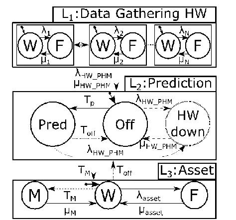
The goal of the proposed verification approach is the verification of prognostics requirements at independent and dependent design layers. When designing a prognostics system, we differentiate three design layers (L): L1: data-gathering hardware; L2: prognostics software model; and L3: RUL

prediction of the asset. Requirements for each of these design stages will be different. However, their inter-dependencies need to be taken into account (i.e., L1L2L3).

Throughout the paper we will assume that L1 fails in

omission failure mode, i.e., hardware fails to provide the data when required. This failure will prevent the prognostics software model (L2) from making predictions and accordingly, intelligent condition-based maintenance actions cannot be undertaken for the asset under study (L3).

Fig. 1 shows the generic pattern for prognostics parameter specification. Dashed connections and states indicate dependencies between modules. The data gathering module depends on the application-specific hardware. Depending on whether the data gathering architecture has failed or not, it will affect the prediction module. In Fig. 1 this is represented with an equivalent failure and repair rate of the hardware system failure (λHW_PHM, μHW_PHM). In reality, these failure and repair rates will be computed using reliability analysis techniques such as Fault Tree analysis [11].

The prediction module will transit between prediction (Pred) and failed states (HW down) according to the deterministic prediction instants of the prognostics module (Tp) and failure rates of the data gathering architecture respectively.

The asset module transits among working (W), failed (F), and maintenance (M) states. If there is no prognostics information, the maintenance time TM is defined by the default preventative maintenance: TM = TPrev, where TPrev designates the preventive maintenance rate. However, if prognostics predictions are performed, TM is defined with the RUL estimation of prognostics. Typically it will be defined by a safety factor SF so that TM = RUL-SF.

The failure of the data-gathering architecture causes the failure of the prediction block and accordingly, prognostics predictions cannot be performed without real up-to-date data.

Fig. 2 shows the overall verification approach. The core of # CSL Meaning

1 P=? [F<t prop1] Prob. of prop1 is true eventually before t

2 P=? [G[t1,t2] prop1] Prob. globally prop1 is true within the time instant [t1,t2]

3 P=? [prop1U<=t prop2] Prob. of prop2 not being true until prop1 is not true in the interval [0,t]

4 R{“oper”}=? [C<t] Expected cumulative operational time

5 R{“time”}=? [F prop ] Time accumulated until prop is satisfied

the proposed approach is the prognostics system specification depicted in Fig. 1. For the specification of the data-gathering architecture, the Minimal Cut Set (MCS) is defined [11] in conjunction with the specification of failure and repair rates of components. The MCS defines the minimal and sufficient combination of component failures that cause the failure of the hardware architecture. As for the prognostics algorithm specification, prediction time Tp, RUL estimation, and default preventive maintenance period Tprev are taken into account. Finally, for the specification of the asset behavior, failure and repair rates of the asset under study are considered (λAsset, μAsset respectively). Note that the failure rate of the asset will determine the ground truth estimation.

The state-based specification in Fig. 1 is specified in PRISM and requirements over this model are specified using CSL in the same modelling formalism. The final outcome of the proposed framework is the probabilistic argumentation of whether the prognostics application meets design requirements. If these are not satisfied, the prognostics algorithm prediction needs to be reconsidered – assuming that the data gathering architecture is a fixed design decision.

V. CASE STUDY

Transformers are the most expensive asset in the power system, and critical to meeting network performance targets. Therefore condition monitoring and prognostics of transformers can lead to a cost-effective maintenance strategy.

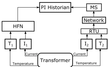
A. Data Gathering Architecture

A common data-gathering architecture for transformers uses temperature and current sensors. It may comprise a redundant data gathering scheme, employing a High Frequency Network (HFN) where available (e.g., critical substations), supported by the lower frequency SCADA network. The SCADA platform includes a Remote Terminal Unit (RTU), in the substation reporting to the central Master Station (MS). Both SCADA and higher frequency data are then archived, using a system such as a PI Historian (cf. Fig. 3).

Fault Tree analysis of the architecture in Fig. 3 identified the combination of component failures that lead the system to failure. This is the Minimal Cut Set (MCS) function:

MCS = PI ˅ (T1˄T2) ˅ (I1˄I2) ˅ [HFN˄(MS˅Net˅RTU)] 

where PI indicates the failure of the PI Historian, Ti and Ii

indicate the failure of the ith _{temperature and current sensor} respectively, Net indicates the failure of the network, and HFN,

MS, and RTU indicate the failure of the identified components. For the analysis we have used hypothetical failure and repair rates (cf. Table II).

TABLE II. FAILURE AND REPAIR RATES OF HARDWARE COMPONENTS

Component λ (m-1_{) µ (m}-1₎

PI Historian 0.001 0.25

Temp. sensor, current sensor, MS, RTU, HFN 0.01 0.25

Network 0.0001 0.25

B. Transformer Prognostics Model

Transformer aging involves deterioration of the paper insulation due to temperature. One model which relates temperature to rate of change of paper degradation is found in IEEE Standard C57.91, which defines an aging acceleration factor. This can be rearranged to give a particle filter process model, by converting it into a recurrence relation for remaining paper life [12]:

Lt = Lt-1 - exp(15000/383-15000/(273+Θ_Ht)) + ut 

where t is the time index in hours, Lt is RUL at time t, Θ_Ht is hotspot temperature at time t, and ut is process noise.

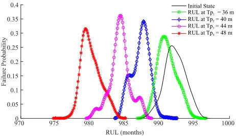
Based on this model we have performed predictions at different time instants (Tp) obtaining RUL estimations shown in Fig. 4.

Ideally the probabilistic model-checker would have the possibility to model the PDF obtained with the particle filter because it includes uncertainty information [13]. However, given that there is no possibility to model these PDFs directly, we adopt the following approximation λ≈1/RUL [14]; that is, we use the mean RUL with maximum and minimum deviation as the failure rate parameters of the exponential distribution.

The RUL prediction results (in months) are as follows: T_p1 (36m) = 992.5 ± 2.89 m; T_p2 (40m) = 987 ± 2.64 m;

Fig. 2. Probabilistic model-checking of prognostics systems.

T_p3 (44m) = 984.3 ± 2.76 m; and T_p4 (48m) = 979.3 ± 3.05 m. See [12] for more details of the particle filter model.

C. Prognostics Requirements Verification

Focusing on the verification of the hardware, these are the analyzed requirements: “Probability that eventually the data gathering system fails in [0, T]” implemented via property #1

in Table I; “Probability that the MCS occurs for more than T time units in order to avoid intermittent failures”; analyzed via

property #2 in Table I; and “Probability that the first failure of the HW architecture occurs in the [T, T+Ttransient] period”

verified via property #3 in Table I. Fig. 5 shows the results.

As Fig. 5 confirms, the difference between transient and permanent failures is evident, i.e., transient failures lead to higher failure probabilities. Besides, we can see that the first failure occurrence is more likely to occur in the first half of the time interval. These results can trigger redesign decisions – for instance, if the designer needs to postpone the first failure occurrence, different hardware modules will be needed to satisfy the design requirements.

With probabilistic model-checking we can evaluate other properties of interest such as maximum operation time of the data gathering architecture. This is defined using PRISM filter command as follows [6]: filter(max, R{"time"}=? [F MCS],!MCS); which informally means: maximum time to failure (MCS) starting from an operative state (!MCS). This property gives as a result of 92.72 months using the values in Table II.

As for the metrics of the prognostics prediction module, we

will focus on false positive and negative metrics. Recall that we have assumed that the data-gathering hardware architecture fails in omission failure mode. Accordingly, the effect of the omission failure on the particle filtering and prognostics metrics needs to be taken into account.

The hardware omission failure provokes the incorrect RUL prediction of the particle filtering model. Namely, the RUL prediction will not include the aging that has occurred during the data outage. Therefore, this failure will have a direct effect on false negative metric. That is, it will increase the false negative rate because the particle filter will predict an RUL which does not take into account data outage periods.

In PRISM rewards can be used to define False Positive (FP) and False Negative (FN) metrics. Assuming that asset=1

identifies failed state, asset=2 identifies maintenance state,

pred=2 identifies HW down state in the prediction module (cf. Fig. 1), and CIX identifies the confidence interval of the event X, where X = {FP, FN}; we define the following conditions

FN = (asset=1)˄ (RUL+Tp >λAsset - CIFN) ˅ (pred=2) 

FP = (asset=2)˄ (λAsset - (RUL+Tp)) > CIFP) 

When reward equations (3) and (4) are satisfied by the PRISM reactive modules they will be increased by a unit. For the asset under study we have used the following reliability figures (in months): λAsset = 1/1038 m-1 (transformer failure rate); μm = 0.1 m (maintenance time); μAsset = 1 m (repair time);

CIFP = 10 m; CIFN = 4 m, and SF = 4 m (safety factor).

After specifying false positive and false negative rewards in PRISM using the property #4 in Table I, Fig. 6 shows the obtained results. If the designer has a threshold for an acceptable rate of FP and FN events this would lead to identifying if these values are acceptable or not.

For the FP events we have used different prediction results from Fig. 4 including their deviation. After the prediction at the time instant Tp = T_p2-dev, the prognostics predictions become accurate enough to avoid false positive event occurrences.

For the FN event we have used the mean RUL prediction value at T_p1. Fig. 6 (b) shows the difference between the metric with and without the hardware omission failure effect. The incorporation of the hardware omission failure enables accounting for the uncertainties that may arise in the prognostics application environment.

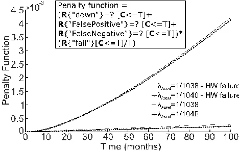
The failure of the data gathering hardware architecture causes the failed prognostics prediction, which in turn leads to a non-updated maintenance schedule at the asset level. We have defined a penalty function using rewards which includes the effect of downtimes (i.e., asset in failed state sums 1 while in maintenance state sums 0.5), FP, and FN events multiplied by the probability of failure of the asset under study.

Fig. 7 shows the effect of different failure rates of both the transformer and data gathering hardware failures. Apart from the uncertainty arising from the application context, the specification of the failure rate of the asset (or ground truth) Fig. 4. Transformer RUL prediction at different prediction times Tp.

has uncertainties too. The ground truth is estimated either under some specific conditions or it is an average failure behavior. Therefore, when using it as a reference failure model, uncertainty estimations should be included. In this case study uncertainty in the ground truth value makes little difference.

VI. CONCLUSIONS &FUTURE WORK

In this paper we have investigated the use of probabilistic model-checking for the formal verification of prognostics system requirements.

The main limitation for the specification of prognostics results is the lack of mechanisms to model any probability density function. This would allow the inclusion of the uncertainty information of the prognostics results and evaluation of other prognostics metrics.

However, the advantages offered by the proposed framework are worth considering: (a) a single integrative framework including hardware/software behavior; (b) formal specification of the system behavior and design requirements for an exhaustive formal verification; and (c) mechanisms to automate the quantification of prognostics metrics and compare prognostics approaches with respect to design requirements.

Future work for the formal verification of prognostics requirements will include the analysis of other probabilistic techniques to overcome the stated limitations and automating

the connection between prognostics and formal models.

REFERENCES

[1] J. I. Aizpurua and V. M. Catterson, "Towards a methodology for design of prognostics system," presented at the Annual Conference of the Prognostics and Health Management Society 2015, San Diego, 2015. [2] T. Liang, M. E. Orchard, K. Goebel, and G. Vachtsevanos, "Novel

metrics and methodologies for the verification and validation of prognostic algorithms," in Aerospace Conference, IEEE, 2011, pp. 1-8. [3] A. Saxena, J. Celaya, E. Balaban, K. Goebel, B. Saha, S. Saha, et al.,

"Metrics for evaluating performance of prognostic techniques," in Int. Conf. on Prognostics and Health Management.2008, pp. 1-17.

[4] S. Sankararaman, "Are current prognostic performance evaluation practices sufficient and meaningful?," presented at the Annual Conf. of the Prognostics and Health Management Society, Texas, 2014. [5] C. Baier and J.-P. Katoen, Principles of model checking: MIT press

Cambridge, 2008.

[6] M. Kwiatkowska, G. Norman, and D. Parker, "PRISM 4.0: verification of probabilistic real-time systems," presented at the Proceedings of the 23rd international conference on Computer aided verification, 2011. [7] B. J. Taylor, M. A. Darrah, and C. D. Moats, "Verification and

validation of neural networks: a sampling of research in progress," in Intelligent Computing: Theory and Applications, 2003, pp. 8-16. [8] J. Schumann, K. Y. Rozier, T. Reinbacher, O. J. Mengshoel, M. Timmy,

and C. Ippolito, "Towards real-time, on-board, hardware-supported sensor and software health management for unmanned aerial systems," Int. Jour. of Prognostics and Health Management, vol. 6, 2014. [9] W. Sanders and J. Meyer, "Stochastic Activity Networks: Formal

Definitions and Concepts⋆," in Lectures on Formal Methods and Performance Analysis. vol. 2090, ed: Springer, 2001, pp. 315-343. [10] J.-P. Katoen, M. Kwiatkowska, G. Norman, and D. Parker, "Faster and

Symbolic CTMC Model Checking," in Process Algebra and Probabilistic Methods. Performance Modelling and Verification. vol. 2165, ed: Springer, 2001, pp. 23-38.

[11] W. E. Vesely, M. Stamatelatos, J. B. Dugan, J. Fragola, J. Minarick, and J. Railsback, "Fault tree handbook with aerospace applications," NASA Office of Safety and Mission Assurance, 2002.

[12] V. M. Catterson, "Prognostic modeling of transformer aging using Bayesian particle filtering," in Electrical Insulation and Dielectric Phenomena (CEIDP), 2014 IEEE Conference on, 2014, pp. 413-416. [13] S. Sankararaman, "Significance, interpretation, and quantification of

uncertainty in prognostics and remaining useful life prediction," Mechanical Sys. & Signal Processing, vol. 52–53, pp. 228-247, 2, 2015. [14] D. Banjevic and A. K. S. Jardine, "Calculation of reliability function and

remaining useful life for a Markov failure time process," IMA Journal of Management Mathematics, vol. 17, pp. 115-130, April 1 2006. Fig. 6.Prognostics prediction module metrics: (a) false positive; (b) false negative.