Bubble collapse near a fluid-fluid interface using the spectral element marker particle method with applications in bioengineering

InternationalJournalofMultiphaseFlow90(2017)118–143

ContentslistsavailableatScienceDirect

International

Journal

of

Multiphase

Flow

journalhomepage:www.elsevier.com/locate/ijmulflow

Bubble

collapse

near

a

fluid-fluid

interface

using

the

spectral

element

marker

particle

method

with

applications

in

bioengineering

Christopher

F.

Rowlatt

∗

,

Steven

J.

Lind

SchoolofMechanicalAerospace&CivilEngineering,TheUniversityofManchester,Manchester,M139PL,UnitedKingdom.

a

r

t

i

c

l

e

i

n

f

o

Articlehistory: Received4April2016 Revised22September2016 Accepted24November2016 Availableonline1December2016

Keywords: Bubbledynamics Drugdelivery Sonoporation Spectralelement Markerparticlemethod Bioengineering

a

b

s

t

r

a

c

t

The spectral element marker particle (SEMP) method is a high-order numerical scheme for modelling multiphase flow where the governing equations are discretised using the spectral element method and the (compressible) fluid phases are tracked using marker particles. Thus far, the method has been suc- cessfully applied to two-phase problems involving the collapse of a two-dimensional bubble in the vicin- ity of a rigid wall. In this article, the SEMP method is extended to include a third fluid phase before being applied to bubble collapse problems near a fluid-fluid interface. Two-phase bubble collapse near a rigid boundary (where a highly viscous third phase approximates the rigid boundary) is considered as validation of the method. A range of fluid parameter values and geometric configurations are stud- ied before a bioengineering application is considered. A simplified model of (micro)bubble-cell interac- tion is presented, with the aim of gaining initial insights into the flow mechanisms behind sonoporation and microbubble-enhanced targeted drug delivery. Results from this model indicate that the non-local cell membrane distortion (blebbing) phenomenon often observed experimentally may result from stress propagation along the cell surface and so be hydrodynamical in origin.

© 2016 The Authors. Published by Elsevier Ltd. This is an open access article under the CC BY license ( http://creativecommons.org/licenses/by/4.0/).

1. Introduction

The dynamics of bubble collapse has received substantial at-tention in the literature over the past 100 years. Starting with Lord Rayleigh (1917), who considered the collapse of a spheri-cal cavity in an infinite expanse of incompressible fluid, subse-quent experimental, numerical and analytical studies have high-lighteda complexphysicalprocess, wherepossibleobserved phe-nomenainclude jet formation,pressure shockwave emission and toroidal bubble formation (see, for example, Benjamin and Ellis, 1966; Lauterborn and Ohl, 1997). Research is motivated by the prevalenceofbubblesinnatureandindustryandtheir fundamen-tal role in many fluid systems. Cavitation damage due to bub-blecollapseisnowa well-knownphenomenon, andhasnegative consequencesin anumber ofareas.In biomedicine, forexample, ultrasound mediated drug delivery (Hernot and Klibanov, 2008; Lentacker et al., 2014; Wu and Nyborg, 2008) and shock-wave lithotripsyprocedures(Freundetal.,2009;KodamaandTakayama, 1998) can generate cavitation bubbles that maycause cell death and hemorrhaging in the surrounding tissue, respectively. How-ever, bubbles may also be used to dissolve blood clots (see e.g.

∗ _{Correspondingauthor.}

E-mail addresses: [email protected] (C.F. Rowlatt),

[email protected](S.J. Lind).

Ungeretal.,2002),breakthroughtheblood-brainbarrier(seee.g. Tingetal.,2012)andcleanandsterilisesurfaces(seee.g. Chahine etal.,2016;Songetal.,2004).Numericalstudiesofbubble dynam-icshavebeendominatedbytheboundaryelementmethod(BEM), originally used in this context by Blake et al. (1986, 1987). The methodrequirestheassumptionofirrotationality,which consider-ablysimplifiesthegoverningequations.Whilethisassumptionhas proven effective formoderate to highReynolds numbers(Curtiss etal., 2013;Klaseboer andKhoo,2004a, b) andincases ofweak flow compressibility(Wang,2014;WangandBlake,2010),it pre-cludessomekeyphysicsnecessaryinthemodellingofmultiphase biomedical flows, such as strong compressibility (i.e. ultrasound) andgeneralnon-Newtonianeffects.

Numerical solutions of the full Navier-Stokes equations for bubble dynamics problems have received considerably less at-tention in the literature than boundary elements, most likely due to the increased implementation difficulty and computa-tional time. Shopov and Minev(1992); Shopovet al. (1990)and Shopovetal.(1992)considered afiniteelementapproximationof the incompressibleNavier-Stokes equations,wherethe meshwas fittedto thebubble surfaceandevolvedina Lagrangian manner. Fitting thecomputational mesh to the bubblesurfacecould sub-stantiallyincrease thecomputational time,particularlyunder sig-nificanttopologicalchanges. PopinetandZaleski(2002) produced a well-defined (unfitted) interface over a finite volume grid by

http://dx.doi.org/10.1016/j.ijmultiphaseflow.2016.11.010

sphericalbubblesandtestcasesincludedthebehaviourofa bub-bleunderbothaweakandstrongacousticwave. Wang(2014) sub-sequentlyappliedthecompressibleBEMmodeltobubblecollapse neara rigid wall.During theincompressible phaseof thebubble dynamics, Wang(2014)achievedexcellentagreementwith experi-mentalobservations.Duringthebubblerebound,where compress-ibilityisimportant,theagreementwasan improvementon previ-ousresults(e.g. PopinetandZaleski,2002)butstilldifferedwhen compared to experiments (see their Fig. 7). It is likely that the secondary collapse phase required an amount of compressibility which isbeyond thescope of theBEM model. Intheir boundary elementstudy,(Leeetal.,2007)tookadifferentapproachand ap-proximatedcompressibleeffectsbyincorporatingaloss inenergy (provided by experimental data) during the bubble rebound and found very good agreement with experimental results, including the captureoftheelusive counterjet. Müller etal.(2010) consid-ered collapse ofa gas filled bubble neara rigidwall using a fi-nite volume techniqueforthe compressible Eulerequations. They showedthatwhenabubblecollapsesneararigidwall(inthe ab-sence of viscosity, buoyancy and surface tension), the compress-ible bubblecontents interactwithreflected pressureshock-waves (causedbytheoscillationofthebubble),producingvorticesinthe gaseous bubblecontents. These vortices rotate inopposite direc-tionsandaredirectedtowardstherigidwall.Thevorticespullthe gaseousbubblecontentsandbubblesurfacetowardstherigidwall producing the well-known toroidal shape and high-speed liquid jet. Importantly,theseareobservationswhichcannot beobtained fromincompressibleandirrotationalsimulationssuchasBEM.The above studies, particularly that of Müller et al. (2010), illustrate theimportanceofcompressibility,eveninsituationscommonly as-sumed to be predominantly incompressible. It is evident that if compressibleeffectsaretobeincludedthenthefullcompressible Navier-Stokes(orEuler)equationsmustbeconsidered.

Lind and Phillips developed a Spectral Element Marker Parti-cle (SEMP) method for fully compressible bubble collapse prob-lems inbothNewtonian (Lind andPhillips,2012) andviscoelastic fluids (Lind and Phillips,2013) with small to moderateReynolds numbers. SEMP uses the marker particle method (Rider and Kothe,1995)totrackthefluidphases.Themarkerparticlemethod is Lagrangian in nature and bears semblance to both the VOF (HirtandNichols, 1981) andthe MAC(Harlow andWelch, 1965) methods. Acolour function Cis determinedby tracking massless markerparticles. Eachparticle isassigneda particularcolour de-pending upon the phase in which it resides, and because a par-ticle offluid willremain of that fluid type (assumingno change inphase),aparticlewillkeepitscolourindefinitely. Within fluid-fluid interface regions, where two (or more) differently coloured sets of marker particles reside, a weighted average is taken of the surrounding particles to determine an interpolated colour at a desired grid point.In this article,SEMP is extended to include

a third phase, that may be used to model deformable biological matter (e.g. cellsor tissue). While there have been a number of worksconsidering bubblecollapse neardeformable surfaces (see e.g. KlaseboerandKhoo,2004b;Ohletal.,2009),fewinclude suf-ficientphysics to modelthecomplex multiphase biomedical pro-cesses that motivate this work. Indeed, the eventual aim is to gaininsights intothe flowmechanisms behindsonoporation (e.g. Lentacker et al., 2014) and microbubble-enhanced targeted drug delivery(e.g. HernotandKlibanov,2008).

This article is structured as follows. The mathematical model and governing equations are introduced in Section 2 with their numericalapproximation discussed in Section 3. Thethree-phase methodisvalidatedin Section 4before anumerical investigation intotheeffectofviscosityandthethicknessofthethird phaseis givenin Section5.Asimplifiedmodelof(micro)bubble-cell inter-actionispresentedin Section6 beforethearticleisconcludedin Section7.

2. The mathematical model and governing equations

Consider atwo-dimensional (2D) domain

,whichcontainsa gas-filled bubble

b of initial density

ρ

b,0, surrounded by fluid

f of initial density

ρ

f,0, placed near a fluid layer

c such that

f=

\

(

b∪

c

)

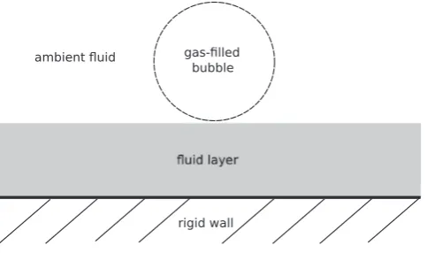
.Notethatallvariableswithindexbwillrefer

tothoseassociatedwiththebubble,thoselabelledfwiththe am-bientfluidandthoselabelledcwiththefluidlayer.Aschematicis givenin Fig.1.

Ingeneral, theequationsgoverningfluidmotionarethe math-ematicalstatementsofconservationofmomentum

ρ

D_Dtu= −

∇

p+

∇

·S, (1)

andconservationofmass

D

ρ

Dt +

ρ

∇

·u= 0,

[image:2.595.318.560.57.200.2]

120 C.F.Rowlatt,S.J.Lind/InternationalJournalofMultiphaseFlow90(2017)118–143

state isrequiredto closethe systemof governingequations. Fol-lowing LindandPhillips (2012), theequation of state istakento betheidealgaslaw,namely

p= c

_{γ ρ}

2 = c¯2

ρ

, (2)

wherec isthe speed ofsound within the medium,

γ

is the ra-tioof specific heats (adiabatic index) and c¯₌c_/√

γ

. The specific heat ratio typically takes values between 1 and 1.7, for a range ofdifferentgasesof variousmolecular weights andtemperatures (White,2010). Thevalue of√

γ

is,therefore,closetoone, andso wetake c¯=c throughoutthispaperasafirstapproximation. De-spiteits simplicity (and limitations), (2) is a useful model (Lind andPhillips,2012;2013).Firstly,itprovidesa reasonablyaccurate thermodynamicdescription ofthebubbles gaseous contents. Sec-ondly,byvariationofasinglemodelparameterone caneasily ex-ploretheeffectofcompressibilityontheflow,andreadilyrecover near-incompressibility,ifrequired.

Theconstitutiveequation,orrheologicalequationofstate,fora compressibleNewtonianfluidiswellknown.Theextra-stress ten-sorisgivenby

S =

η

1

∇

u+

∇

uT

₊

_η

2

(

∇

·u

)

I, (3)

where

∇

u is the velocity gradient, the superscript T denotes the transpose, I is the identity tensor and

η

1,2 are scalar coef-ficients. Commonly,

η

1 is named the (dynamic) shear viscosity coefficient and

η

2 is termed the dilatationalviscosity coefficient. Eq. (3) is the most general constitutive equation for a Newto-nian fluid as it imposes no restrictions on compressibility oron

η

1,2. Often one abides by Stokes hypothesis and sets the bulk viscosity

κ

=

2

3

η

1+

η

2

to zero(Gad-el-Hak,1995). As stated in Lind and Phillips (2012), this implies that the mean mechanical pressurep∗ becomesequivalenttothethermodynamic pressurep in Eq.(1)andthat the extrastress istrace free:_iSii=0.

How-ever,inthisworkStokes’hypothesis isnotadoptedandthemost general form of the compressible Newtonian extra-stress tensor (Eq.(3))isretained.

2.1.Nondimensionalisationofthegoverningequations

This article employs a similar non-dimensionalisation asused in Lind andPhillips (2012): distances are scaled withrespect to initial bubble radius R, densities are scaled with respect to the initial bubble density

ρ

b,0, pressures are scaled with respect to

ρ

b,0V2, where V is a referencespeed of sound(e.g. the speed of soundthroughanidealgas),andstressesarescaledwithrespectto

ρ

b,0V2.Consequently,thenon-dimensionalviscosities

η

∗arescaled accordingto

η

∗₌

η

ρ

b,0VR .

AReynoldsnumbercanbedefinedasRe=1/

η

∗_,butitismore beneficial to refer tonon-dimensional viscosities dueto the sev-eralviscousparameterspresentincompressiblemodels.Therefore, dropping the asterisks and substituting Eq. (2) into Eq. (1), the non-dimensional governing equations for a compressible Newto-nianfluidare:theconservationofmomentum

ρ

D_Dtu= −c2

_∇

_ρ

₊

_∇

_{·S, (4)}

theconservationofmass

D

ρ

Dt +

ρ

∇

·u= 0, (5)

andtheconstitutiveequation

S =

η

1

∇

u+

∇

uT

₊

_η

2

(

∇

·u

)

I. (6)

Asin LindandPhillips(2012),alog-densityformulationis im-plementedwherethegoverningequationsaresolved forlog den-sityq :=ln(

ρ

) andakinematicstress S :=

ρ

T .Thestandard and log-densityformulationsofthegoverningequationsarephysically equivalent, but the log-density formulation is convenient as the coupled mass and momentum equations become predominantly linearforconstantkinematicviscosity(BolladaandPhillips,2007; 2008). There are also numerical stability benefits for multiphase flows aspotentiallylarge densitydifferencesacross interfacesare scaleddowninmagnitudewhenworkingwiththelogdensity. Ac-cordingly, any subsequent reference to the density orstress will technicallyrefertothelogdensityandkinematicstress,asdefined above.

3. Numerical solution of the governing equations

3.1. Timediscretisation

In this article, a semi-Lagrangian approximation of the mate-rial derivative is used for both the conservation of momentum andmassequations(Eqs.(4)and (5)),(BolladaandPhillips,2007, 2008). A notable feature of the semi-Lagrangian scheme is that it can relieve the time step (CFL) restriction. When the semi-Lagrangian scheme is used in conjunctionwith the spectral ele-ment method(as isthe casehere), therestriction on thesize of thetime-stepisduetoaccuracyconsiderations ratherthan stabil-ity(KarniadakisandSherwin,2005). Suchaccuracyconsiderations canbeinformedbytheworkof FalconeandFerretti(1998),where itisshown(fortheone-dimensional advection-diffusionequation withafiniteelementtypemethod)thattheoverallerrorof semi-Lagrangianschemesisgivenby

O

tk₊

xN+1

t

(7)

where N is the polynomial degree of the spatial approximation andkistheorderofthebackwardintegrationstep.Inthisarticle, weemploy afirst-orderLagrangian approximationofthematerial derivative:

Du

Dt ≈

un+1

₍

_xn+1

₎

_−un

₍

_xn

₎

t = f

(

u

n+1

₎

_{, (8)}

where u n

₍

_x

₎

_=u

₍

_{x ,t}n

₎

_{isthevelocity ofafluidparticle x attime}

tn_=n

_{t, n=1,...,N}

t (where Nt is the total number of time

steps), x n_=x

₍

_tn

₎

_{denotesthepositionofafluidparticleattimet}n

andfistherighthandsideofthemomentumequation.Given u n_,

we wish tosolve Eq.(8)implicitlyfor u n+1 _{foreach nodalpoint.} Hence, in order to approximate the material derivative, the pre-vious position x n _{ofthe fluid particlethat moves ontothe nodal}

point x n+1 _{isrequired,inadditiontothevelocity u} n+1_.Inthis ar-ticle, we employa second-order mid-pointrule todetermine the previousposition x n_{,whichistypicalforsemi-Lagrangianschemes}

The spectral element method (SEM) was first proposed by Patera (1984) to extend the application of spectral methods to problems definedin complexgeometries. SEM hasthe geometric flexibility ofa finite elementmethod (FEM)withthe accuracyof a spectral method and therefore, in principle is similar to hp -FEM. It is well-known that the SEM should perform better than traditionalfiniteelementsbothintermsofaccuracyandefficiency providedthesolutionissufficientlyregularandtheacceptederror levelissufficientlystringent(Patera,1984).

3.2.1. Weakformulation

As stated at the beginning of this section, the whole domain

⊂R2 _{containsthe bubble}

b, the fluid layer

c and the

am-bientfluid

fsuchthat

f=

\

(

b∪

c

)

.Thespectralelement

methodisbasedonsolvingthegoverningequationsintheir equiv-alentweakform.Thus,thedependentvariables u ,qand T are cho-senfromthefollowingfunctionspaces:

u ∈ V :=

H01

()

2

, q∈ Q := H1

()

, T ∈ T :=

H1

()

2_s×2,

where H1₍

_{) is a Sobolev space whose elements, and their first} weakderivatives,areinL2₍

_{)(AdamsandFournier,2003),H}1

0

()

containsanyelementsofH1₍

_{)whosetracetotheboundary}

∂

_is zeroand

H1

₍₎

2×2

s containsall2×2,symmetrictensorswhose

componentsareelementsofH1₍

_{).Multiplyingthestrongformof} thegoverningequationsby anappropriate testfunctionand inte-grating yields the following semi-discrete weak formulation:find

(

u ,q,T

)

∈V×Q×T suchthat

u−un

t ·

v

d

+ T :

∇

v

d

= c

2

q

∇

·

v

d

+

∇

q·T ·

v

d

∀

v

∈ V, (9a)

_q−qn

t +

∇

·u

pd

= 0

∀

p∈ Q , (9b)

T:Wd

−

μ

1

∇

u:

(

W + W

T

₎

_d

=

μ

2

(

∇

·u

)

tr

(

W

)

d

∀

W ∈ T , (9c)

wheretr(W )isthetraceofatensor.

3.2.2. Spatialdiscretisation

In the spatial discretisation of the weak formulation (9) us-ing the spectral element method, it is necessary to choose con-forming discrete subspaces _VN⊂V, QN⊂Q andTN⊂T.The

do-main

isdividedintoanumberofnon-overlapping, conforming, convex, quadrilateralspectral elementslabelled

_α,β.The

coordi-nates(

α

,

β

)labeleachspectralelementsuchthat

α

₌0_,...,

α

ˆ and

ibility conditions for the velocity and pressure (not density) ap-proximationspacesareknownforincompressibleflow,we empha-size that no inf-sup stabilityissues havebeen seen in our com-pressible computations. Each spectral element is mapped to the parent domain D=[−1,1]×[−1,1] using a transfinite mapping, F , of Schneidesch and Deville (1993), where for each point

ξ

=

(ξ

,

ζ

)

∈D there exists a point x =

(

x

(ξ

,

ζ

)

,y

(ξ

,

ζ

))

∈

α,β, such that x =F

(

ξ

)

andtheverticesof

_α,β aregivenby x 1,...,x 4.The velocity,densityandstressareapproximatedoneachelement us-ing Lagrangian interpolationthrough a selectset ofnodalpoints, called Gauss–Lobatto Legendre (GLL) points. In one dimension, the

(

N+1

)

GLL pointsarerootsof thepolynomial

(

1−

ξ

2

₎

_L

N

(ξ

)

whereLN isthe Legendre polynomial ofdegree N.Therefore, the

Lagrangeinterpolantcanbeshowntotaketheform

hi

(

ξ

)

= −

(

1−

ξ

2

)

_L

N

(

ξ

)

N

(

N+ 1

)

LN

(

ξ

i

)(

ξ

−

ξ

i

)

(11)

where

ξ

i, i=0,...,N are the GLL points. The Legendre

polyno-mials are a subset of polynomial eigenfunctions (Jacobi polyno-mials) of the singular Sturm–Liouville differential operator and it is well known, that the expansion of a C∞ function in terms of these eigenfunctions converges with spectral accuracy (expo-nential rates of convergence). Hence, an expansion in terms of the Lagrange interpolants (11) exhibits spectral properties, while alsonaturallylendingitself to Gauss–LobattoLegendre numerical quadrature.Thisisanimprovementovertraditional(h-type)finite elementmethods,whichexhibitalgebraicratesofconvergence.

In2DtheGLLpointsforma

(

N+1

)

2_{gridwithineachelement,} interpolation overwhich yields the representationof each veloc-itycomponent,stresscomponentanddensityovertheparent ele-ment

ua

₍

_ξ

_,

_ζ

₎

₌ N

i=0

N

j=0

ua

i,jhi

(

ξ

)

hj

(

ζ

)

, (12a)

Ta,b

₍

ξ

_,

ζ

₎

₌ N

i=0

N

j=0

T_ia_,j,bhi

(

ξ

)

hj

(

ζ

)

, (12b)

q

(

ξ

,

ζ

)

=

N

i=0

N

j=0

qi,jhi

(

ξ

)

hj

(

ζ

)

, (12c)

whereua i,j,T

a,b

i,j andqi,j aretheapproximationstou

a_,Ta,b_andqat

eachGLLpoint(

ξ

i,

ζ

j),respectively.Formoredetailsregardingthe

spectralapproximation,thereaderisreferredtothemonographof KarniadakisandSherwin(2005).

Theintegralsintheweakform (9)areapproximatedusingthe Gauss-LobattoLegendrequadraturerule

1

−1 1

−1f

(

ξ

,

ζ

)

d

ξ

d

ζ

≈

N

i=0

N

j=0

122 C.F.Rowlatt,S.J.Lind/InternationalJournalofMultiphaseFlow90(2017)118–143

where the weights wi are chosen so that the quadrature rule

is exact for polynomials of degree less than or equal to 2N−1 (Owens andPhillips, 2002). The fullydiscrete equationsare then obtainedby inserting the variable expansions (Eq. (12)) into the weakform (Eq. (9)) andapplying the above quadraturerule. For detailsofthefulldiscretesystem,thereaderisreferredto Lindand Phillips(2012).

3.3.Themarkerparticlemethod

The marker particle method is a Lagrangian scheme to track multiplefluid phasesandinterfaces. A large number ofparticles placedwithinthedomainactasmarkers,providingtheidentityof thefluidatapointintimeandspace.Theapproachwasfirst sug-gestedby Rider andKothe (1995) andcompares favourably with VOF and level set methods. Particular benefits include the ab-senceofnumericalmassdiffusion andnumericalsurfacetension, and the ability to handle severe topological changes with ease. Furthermore,the scheme is straightforward to implement andis very robust (Rider and Kothe, 1995). It has been subsequently applied in Newtonian drop dynamics studies by Bierbrauer and Zhu(2007)and BierbrauerandPhillips(2008),andthebubble dy-namicsstudiesof LindandPhillips(2012, 2013).

Thewholedomain

isfilledwithinitiallyequallyspaced par-ticles-aspecified numberperunit area. Everymarkerparticlep isinitially located ata uniqueposition (xp,yp) andisassigneda

colour,oridentity,Cm

p definedby

Cm

p =

1 ifparticle pisinfluidm,

0 ifparticle pisnotinfluidm. (13)

Assuming nochangeinphase,particlesinitiallyoffluidmwill remainso indefinitely andwill be advected withfluid m.Hence, thecolourfunction foreachparticlesatisfies theadvection equa-tion,namely

DCm

p

Dt = 0. (14)

Eq.(14)isensuredthroughtheLagrangianupdateofthemarker particles.Astheparticlesremainoffluid m,theycanbe assigned theconstant material propertiesassociated withfluid m, such as fluidviscosities

μ

m.

3.3.1. Gridtoparticleinterpolation

The marker particles, and hence the position of the relative phases, are updated using the velocities calculated on the Eule-rianspectral elementgrid.The velocitiesare interpolatedtoeach markerparticle,andthe particlesare advectedwiththese veloci-tiesaccordingto

u = Dx

Dt.

Thebenefits ofa spectral element formulationmeanthat intern-odalvelocitiescanbefoundwitheaseandhighaccuracyusingthe Lagrange interpolant expansions (Eq. (12a)). Therefore, a particle at(xp,yp)canbeeasilyandaccuratelyassignedavelocity u (xp,yp)

andhenceupdatedinpositionaccordingly.

3.3.2. Particletogridinterpolation

The material properties ofthe fluids, carried withthe marker particles, need to be projected onto the grid before solving the governing equations for the next time step. Following Lind and Phillips(2012),materialpropertiesareassignedtoeach GLLnode usingthefollowingaveragingprocess:

φ

i,j = M

m=1

φ

m_Cm

i,j, (15)

where

φ

m_{denotesamaterialconstantwithinfluidm(forexample,}

viscosity) andMthetotalnumberof separatephases/fluids. Note that,inthisarticle,wehavethreephases;thebubble,theadjacent fluidlayer/cellandtheambientfluid.ThequantityCm

i,jisknownas

theinterpolatedcolourfunctionatthepoint (i,j)andisgivenby

Cm

i,j=

Np

p=1S

(

xp−xi, yp −yj

)

Cmp

Np

p=1S

(

xp−xi, yp−yj

)

, (16)

where Np is the total number of particles and S is a bilinear

weightingfunctiongivenby

S

(

x−xi, y−yj

)

=

1−

x−xi

x

1−

y−yj

y

if0≤

x−xi

x

,

y−yj

y

≤1,

0 otherwise. (17)

Also,notethat,bydefinition

M

m=1

Cm

i,j= 1.

AlthoughCm

i,jisfoundbysummingoverallparticlesinthe

do-main (Eq.(16)), only those within a square of area 4

x

y con-tributetodeterminingtheinterpolatedcolourfunctionatGLLnode (i,j).Theinterpolatedcolourfunctionwillbeweightedtowardsthe colour function (Eq. (13)) of the majorityof particles that are in closeproximitytopoint(i,j).Consequently,by Eq.(15),the mate-rialconstantswillbeweightedtowardthoseofthedominantfluid about(i,j).Ofcourse,thisisimportantonlyinregionsnearthe in-terfacewheretwodistinctfluidtypesarepresent.Withinthebulk offluidm=1,C1

p=1whereasC2p=C3p=0forall particlespnear

(i,j).SoC1

i,j=1andCi2,j=Ci3,j=0;hence

φ

i,j=3m=1

φ

mCim,j=

φ

1.

Wehavesomechoiceinspecifyingthesizeofthesearchsquare 4

x

y.Forregularfinitedifferencemeshes,

xand

yaretaken to be theregular grid spacings. However, the GLL pointsare un-equally spaced. Consequently, it seems prudent to leave the size ofthe search square asan independent parameter,which can be alteredtosuittheproblemathand,undertherestrictionthat

min

(

ξ

i

)

≤

x,

y≤max

(

ξ

i

)

, (18)

where

ξ

i=

|

ξ

i+1−

ξ

i

|

, i=0,...,N−1 is the spacing between

consecutive GLL points. In most instances, setting the search lengths

x,

ytobe anaverageof

ξ

_igivesvery reasonable re-sults.

Notethat throughoutthisarticle,we define additionalmarker particles x _bot, x _int, x top,whichdonotinteractwiththefluidinany

waybutareused solelyto trackthepositionsof thebottomand topofthebubble,aswellasapointinitiallycentral onthe inter-facebetweentheambientfluidandadjacentfluidlayer.

3.3.3. Particleboundaryconditions

Itmaybethecasethatparticlesneartheboundaryinthe cur-renttimestepmaystepoutsidetheboundaryinthenext.To rem-edythis,theparticlesaresimplyreflectedbackintothedomainby theamount atwhich theyexceed it.Thisexact approach isused by BierbrauerandZhu (2007)intheir finite differencestudyand by LindandPhillips(2012).

3.3.4. Acommentonsurfacetension

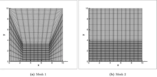
Fig.2. Illustrationof(a)Mesh1;therefinedregionisaboxlocaltothebubbleand(b)Mesh2;therefinedregionisastrip,whichcontainsboththebubbleandthe fluid-fluidinterface.

surface tension does not dominate bubble dynamics, it is physi-cally significant. Its omissioninthiswork partlyresultsfromthe factthatsurfacetensionhasnotyetbeenformallyanalysedwithin themarkerparticleframework:itisanopenquestionwhetherthe best approach is a particle-pairwise interaction force (mimicking molecular generation of surfacetension,see e.g. Tartakovsky and Meakin, 2005) ora Continuum Surface Force (using the continu-ouscolourfunctionasdevisedby Brackbilletal.(1992)).Thisisa non-trivialbodyofworkthatdeservesthoroughinvestigationand theauthors areworkingonthisdirectly.Nevertheless,theresults hereinstillprovideusefulinsightsintobubble-celldynamics,with theabsence ofsurfacetension allowingisolationandclear obser-vationofeffectsduetootherimportantphysics,suchas viscoelas-ticity(see Section6.2).

4. Validation

As is always the case for new numerical code, validation is required to ensure that the method works as expected. The SEMP method has been validated using a time-reversed rotation and multiphase Poiseuille flow examples which are discussed in Appendix C.1 and Appendix C.2, respectively. Here, we validate the bubbledynamicsbyconsidering athree-phase approximation to a two-phase example: bubble collapse near a rigid wall. This is accomplished by setting the fluid layer to havea high viscos-ity so that it approximates the rigid wall. This setup should ob-tain resultsthat arein closequalitativeagreement withthe two-phase examples published by Lind andPhillips (2012). Through-out thissection, let

₌[0_,10]2 _{containan initially circular} bub-ble, withradius R=1 and centre x ˆ=

(

5.0,2.2

)

anda fluid layer

c=[0,10]×[0,1].Weusethesameparameters asthosechosen

by LindandPhillips(2012);thebubblehasdensityq_b,0=ln

ρ

_b,0= 0 and viscosity

μ

_b=10−5_{, while the ambient fluid has density} qf,0=ln

(

4

)

and viscosity

μ

f=10−2. The fluid layer density is

given by qc,0=qf,0 whilst the viscosity is

μ

c=103. The

simula-tionswererununtilT=10withatimesteplength

t=5×10−3. The mesh used in this section is the same as the one used by Lind andPhillips (2012) andis depictedin Fig.2a, where N=8,

α

max=

β

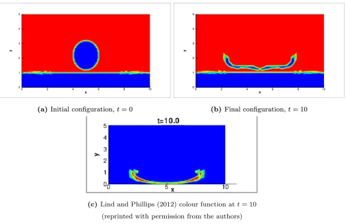
max=9.Theinitialconfigurationofthistestcaseisshown in Fig.3a.

Fig.3b illustrates the colourfunction at theend ofthe simu-lationt=T=10.Clearly, abroadjet hasformed whichimpinges on the fluid layer and pushes the bubble contents out towards thesidewalls.Eventhoughtheviscosityofthefluidlayerisvery high,thecentreofthefluidlayerinterfacedoesmoveslightly up-wardsasthesimulationprogresses.Nevertheless,theresultsarein goodqualitativeagreementwiththetwo-phaseresultsof Lindand Phillips(2012)depictedin Fig.3c.

5. Numerical investigation

Thissection isdedicated tothe numericalinvestigationof the collapseof a gas-filled bubble near a fluid-fluid interface witha rigidbacking,whereboththeambientfluidandthefluidlayerare Newtonian. As mentioned in the introduction, the SEMP method wasdeveloped for flows with smallto moderateReynolds num-ber, orequivalently,when thedensitydifference across phasesis small.To theauthors’ knowledge, theseare the only results (ex-perimental or numerical) for low inertia bubble collapse near a fluid-fluidinterfacebackedbyarigidwall.Intheinterestsof clar-ifying the effect ofkey parameters on dynamics,this section fo-cuses primarily on the effect of viscosity, and accordinglyomits anyeffectsduetoappliedultrasound,buoyancyorsurfacetension. Inthe Appendix A,wedemonstrate thatthe bubbledynamicsdo notchange underap-refinementover areasonablephysicaltime (O(1)timeunits).Here,weconsidervariationsinboththeambient fluidviscosityandthefluidlayerviscositybyseparatingtheresults intotwo parts: whenthe ambientfluid viscosityis lessthan the fluidlayer viscosity,

μ

f<

μ

c andvice-versa,

μ

f >

μ

c.Finally,we

considertheinfluencetherigidbackinghasonthecollapse. Throughoutthis section, the domain

₌[0_,10]_×[0_,10] con-tains a gas-filled bubble,

b, and a fluid layer,

c, so that the

ambientfluid occupiesthe domain

f=

\

(

b∪

c

)

. With the

[image:6.595.51.559.57.307.2]

124 C.F.Rowlatt,S.J.Lind/InternationalJournalofMultiphaseFlow90(2017)118–143

Fig.3. Colourfunctionat(a)thebeginning,(b)theendofthesimulationand(c)two-phaseresultsofLindandPhillips(2012)(reprintedwithpermissionfromtheauthors).

constantviscosity

μ

b=1×10−5.The fluid layeroccupiesthe

do-main

c=[0,10]×[0,h], whereaheight h=1isassumedin all

subsections except Section 5.3, andhas the same density as the ambientfluid,i.e.qc,0=ln

(

4

)

=qf,0.Thetimesteplengthisgiven by

t₌5_×10−3_.Notethatc¯2_=1000.

5.1.Ambientfluidviscositylessthanfluidlayerviscosity

In this section we considerthe case where theambient fluid viscosityislessthantheviscosityofthefluidlayer.Inthissection werestrictourselvestothetimeperiodt=0,...,0.5,because,as indicated in Appendix A, the mostinteresting dynamics seemto occurwithinthisperiod.

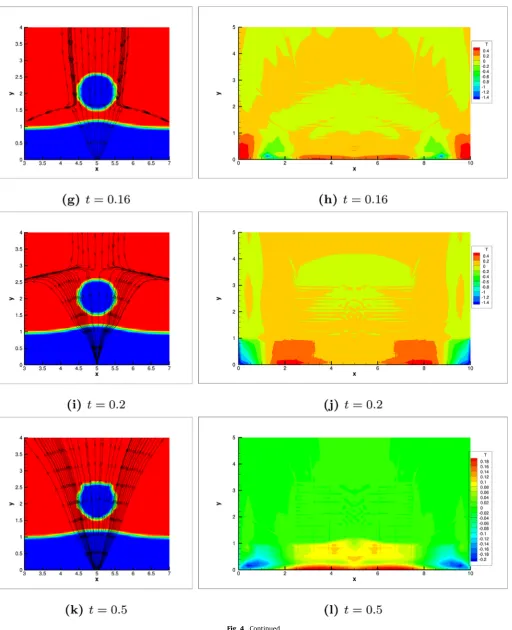
Fig. 4a–k(leftcolumn) illustratethe colourfunction, and spe-cificvelocitystreamlines,attimest=0.04,0.08,0.12,0.16,0.2and 0.5 for material parameters

μ

f=10−3 and

μ

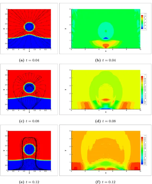
c=10−1. All the

streamlinesdepictedinthissection, andlaterinthearticle,were chosenduringpost-processingusingTecplot.Theinitial configura-tion is thesame as depicted in Fig. 3a. At t=0.04, the velocity streamlinesclearlyillustratethat the bubblehascollapsed spher-ically, drawing the fluid-fluid interface upwards to the bubble.It will be shown later, that this initial collapse phase is controlled primarilybythepressuredifferencebetweenthebubbleand ambi-entfluid,withverylittledependenceonviscosity.Thebubblethen goesthrough an expansion phase which can be seen att=0.08 wherethevelocitystreamlinesclearlyillustratesataperingmotion. Thisexpansionpushesthecentreofthefluid-fluidinterface down-wards slightly before the bubble is elongated towards the fluid-fluidinterface (as a resultofthe taperingmotion), whichcan be seenatt=0.12.Thiselongationiscommonlyseeninbubble cav-itation problems and may be accompanied by jet formation. No

jet is seen here, however,dueto rapid equilibrationof pressures inside andoutsidethebubbleafter theinitial collapse. The elon-gation ofthe bubble occursdue to a Bjerknes-style migration of the bubble (towardsthe more rigidlayer). This migration causes thelayertocompressslightlyandthenrebound,flatteningthe un-dersideofthebubbleatt₌0_.16and0.2. Fromthenon,the bub-bledynamicsapproachasteadystate,withnosignificanttemporal changeindynamics.Smallperturbations canbe seen inthe bub-blesurfaceatt=0.5(andmoreclearlyin Fig.5a). Asmentioned, thesearise dueto an absenceofsurfacetension,but mayevolve intoun-physicalflowfeatures atlatertimesastheirsmallscaleis under-resolved by thegrid. Forlarger viscosityvalues,these per-turbationsare dampenedentirely(see Fig.5) withlong-term sta-bilityevident,asdemonstratedin Fig.A21a.

[image:7.595.42.547.60.387.2]

[image:8.595.47.560.77.698.2]

126 C.F.Rowlatt,S.J.Lind/InternationalJournalofMultiphaseFlow90(2017)118–143

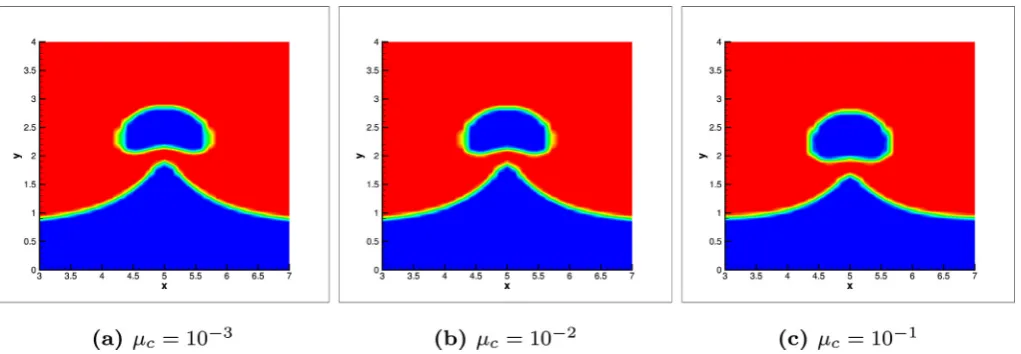
[image:9.595.39.552.81.712.2]

Fig.5. Colourfunctionforμf=10−3,10−2,10−1,μc=1.0whent=0.5.

Fig.6. Colourfunctionwithvelocitystreamlinesforμf=10−1,μc=10−3fort=0.2,0.5,10.

isalsoevident that,asthesimulationprogress,thelargest magni-tudesofstressareseenattherigidwall.Weinvestigatethe influ-enceoftherigidwall later inthearticle,butnote thismayhave significant implications forbubblecleaning processes(ifthe fluid layer were to be a model ofsome unwanted material deposit or contaminant).

5.2. Ambientfluidviscositygreaterthanfluidlayerviscosity

In this section, we assume that the viscosity of the ambient fluidisgreaterthantheviscosityofthefluidlayer. Fig.6illustrates the colour function, and specific velocity streamlines, at times t=0.2,0.5,10.0formaterialparameters

μ

f=10−1 and

μ

c=10−3

(whicharetheoppositeoftheprevioussection).Plotsofthecolour functionattimest=0.04,...,0.16havenotbeenincludedasthe motionofthebubbleisremarkablysimilartotheprevioussection andtherefore,thediscussion forthesetimeswillnotbe repeated here. Intheprevious section,anear-steadystate wasattained(at t ≈0.2)whereonly smalloscillations andmigrationsofthe bub-blewereseen,butsurfaceperturbationswerevisibleduetosmall viscosities. Here,however,the bubbleshape remainssmootherat t=0.2 and t=0.5 dueto the larger ambientviscosity and con-sequently,asdiscussed inthe Appendix A, thesimulation isable to run formuch longer times. Fig.6c illustrates the colour func-tion atthe later time oft=10.It is clearthat the fluid-fluid in-terfaceiscontinuingtopushupwardsintothebubbleafterits re-bound;afterallitnowhasalower viscosityandbetterretainsits momentum, initiallygeneratedby thebubblecollapseinthe

ear-lierstages.Itisclearfromthevelocitystreamlines,thatsmall vor-ticesare createdinsidethebubbleandalsoinsidethefluid layer. Brujanetal.(2001)demonstratedthatwhenalaser-generated cav-itationbubblecollapsesnearanelasticmaterial(inertiadominated collapse),anejectionoftheelasticmaterialintotheambientfluid canbeseen. Asimilarphenomenonisseen here,howeverdueto theloweramountofinertiaintheseexamples,thejet-likegrowth ofthefluid-fluidinterfacedoesnotpiercethebubble.

Fig. 7a illustrates contours of the streamline normal stress at timest₌0_.04_,0_.08_,0_.12_,10.Att₌0_.04_,arelativelylargeamount ofnormalstressappearsradiallyaroundthebubbleasitcollapses. This normalstress clearlydissipates outwards att=0.08 during the bubbleexpansion phase.However, note that there is a build upofnormalstressbetweenthebubbleandthelayerwhichagain mayhave implications forcavitation erosion.Also noticethat, as thesimulationprogresses,thenormalstressesthendissipate out-wards andpartly intothe fluid layer while decreasing in magni-tude. Fig.7dillustratesthenormalstressesthatarefoundattime t=10.There is evidence ofstress build-up on eitherside of the crestatthefluid-fluidinterface.Thesestressesaccompanythefluid mechanicalmotionthatdrives theinterface upward.Theyare in-dicativeoftheretardingeffectoftheambientfluidontheupwards jet,andalsolimitanypossiblepenetrationofthenearbybubble.

[image:10.595.49.561.56.238.2] [image:10.595.44.569.56.436.2] [image:10.595.54.559.249.435.2]

ef-128 C.F.Rowlatt,S.J.Lind/InternationalJournalofMultiphaseFlow90(2017)118–143

Fig.7. Streamlinenormalstressforμf=10−1,μc=10−3fort=0.04,0.08,0.12,10.

Fig.8. Colourfunctionforμc=10−3,10−2,10−1,μf=1.0whent=10.

fect of varying viscosity is quite small,but still noticeable, with decreaseddeformation inboth the interfaceand thebubbleseen for

μ

c=10−1.

5.3.Fluidlayerheightinvestigation

This section is concerned with a numerical study of the in-fluence of the rigid wall which backs the fluid layer. Analogous tothe previous section, the domain

=[0,10]×[0,10] contains a gas-filled bubble,

b, and a fluid layer,

c, so that the

am-bient fluid occupies the domain

f=

\

(

b∪

c

)

. The bubble

centre is positioned at x ¯ (which varies depending on the layer height)withaninitialradiusR=1.Thebubblescontentsare mod-elledasacompressiblefluid withlog-densityqb,0=0anda con-stantviscosity

μ

_b=1_×10−5_{.Thefluidlayeroccupiesthedomain}

c=[0,10]×[0,h](wheretheheightisgivenbyh=0.3,5.0)and

[image:11.595.41.553.56.395.2] [image:11.595.40.551.419.596.2]

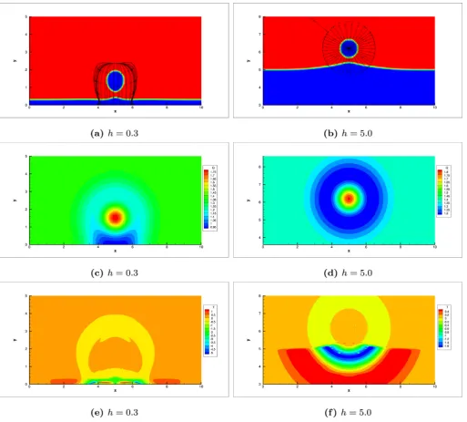
Fig.9. Illustrationofthecolourfunctionwithvelocitystreamlinesatt=0.08(toprow),densitycontouratt=0.04(middlerow)andstreamlinenormalstressatt=0.08 (bottomrow)forμf=10−3,μc=10−1withthefluid-fluidinterfaceatheightsh=0.3,5.0.

5.3.1. Ambientfluidviscositylessthanfluidlayerviscosity

Throughout this subsection, we let

μ

_f=10−3 and

μ

c=10−1.

A comparisonofthecolour function,densityandstreamline nor-malstressforthetwocellheightsquotedabove,isconsidered.The densityisplottedinplaceofthefluidpressure,onthe understand-ingthatthetwoareequivalenttowithinamultiplicativeconstant throughthelinearequationofstate (2).Bychoosingasmallanda largefluidlayerheight,h,wecaneasilyassesstheinfluenceofthe rigidwallbackingthelayer.

Fig.9aandbillustrateacomparisonofthecolourfunction(and specific velocity streamlines) atinterface heightsh=0.3 and5.0. The plots are taken at time t₌0_.08 as the majority of the dy-namics occur early onthe simulation.The difference in the bub-ble shape atthe differentheightsis immediatelyobvious.At the smallerheight, Fig.9a,thebubbleelongatestowardstherigidwall wherethevelocitystreamlinesclearlyillustratesataperingmotion (thisbehaviourwasseenintheprevioussections;seeforexample, Fig. 4c).Whilstat thelarger height, Fig.9b,the bubblecollapses sphericallyascanbe seenfromthe velocitystreamlines.The

rea-sonforthe substantialdifference inbubbleshapescanbe imme-diately seen in the corresponding density contours illustrated in Fig.9candd. Fig.9cshowsthatthereisaregionoflowerpressure on the rigidwall in the region directly beneaththe bubble. Due totheabsenceofbuoyancyandsurfacetension,thepressure gra-dientisthedriving forceforthebubbleelongationandmigration towards thewall. Onthe other hand,at a greaterheight, Fig. 9d showsthat theregionoflow pressureiscontainedinan annulus around the bubble, which dissipates outwards as the simulation progresses;meanwhile the bubblecontinues near-spherical oscil-lationsofdecreasingamplitude.Clearly,thefluidlayerthicknessis sufficientlylarge so asto minimiseany effectofthe wall on the bubble.

[image:12.595.49.563.54.517.2]

130 C.F.Rowlatt,S.J.Lind/InternationalJournalofMultiphaseFlow90(2017)118–143

Fig.10. Colourfunctionwithvelocitystreamlinesforμf=10−1,μc=10−3att=7.0withthefluid-fluidinterfaceatheightsh=0.3,5.0.

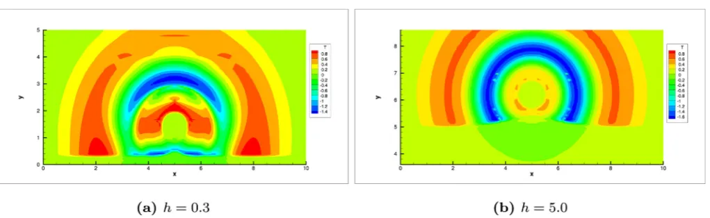
Fig.11. Streamlinenormalstresscontourforμf=10−1,μc=10−3att=0.08withthefluid-fluidinterfaceatheightsh=0.3,5.0.

amannersimilar tothe density/pressure,butwithnotablylarger magnitudesfound within the fluid layer. Thisis expected asthe fluidlayer isofa largerviscosity (bysome twoorders of magni-tude).

5.3.2. Ambientfluidviscositygreaterthanfluidlayerviscosity Following on from the previous subsection, we swap viscosi-tiesandlet

μ

f=10−1 and

μ

c=10−3.Itwasillustratedinan

ear-lier section, that the increased ambient fluid viscosity increases thelifetimeofthebubble.Therefore, Fig.10a andbillustrate the colourfunctionattimet=7.0atinterfaceheights0.3and5.0, re-spectively.Immediately, one seesthe effectthe rigidwall hason thefluid-fluid interfaceandbubble shape.Ata height ofh₌0_.3_, ajetformsinthefluid-fluidinterfacewhichismoreroundedand elongatedthan ata heightof h=5.0.Thefluid-fluid interface, at h=0.3,penetratesalittlefurtherintothebubblewhencompared totheh=5.0case,mostlikelyduetotheincreasedpressurebuild up(andsubsequentrebounddrivingforce)inthesmallerlayerof fluid.Consequently,atthe smallerheight,thebubblecanbeseen to bend around the fluid-fluid interface much more significantly whencomparedtothelargerheight.Itisknownthatwhena bub-bleoscillatesnearaneighbouringcell,microstreamingisproduced inthe surroundingfluid (Wu, 2002). This microstreamingcan be clearlyseenin Fig.10aandb.However,wenotethatthereisvery littleproductionofshearstressassociatedwiththesemicrostreams duetotheirrelativemagnitudebeingsmall_≈O

(

10−2

)

.

In order to draw comparisons with the previous section, the streamlinenormal stress attime t=0.08 is nowconsidered. We donot considercomparisonsforthecolourfunctionordensityas resultsare found to be near-identical to theprevious section for t≤ 0.08. Fig. 11a andbillustratethe streamlinenormalstress at

interfaceheights0.3and5.0,respectively,fortimet=0.08. Com-paredto the previous section, the largestbuild up stress is now seenin theambientfluid. Itisclearfrom Fig. 11a thatthere isa smallbuild upofnormalstress onthe fluid-fluidinterface which has possible implications for cell functionality, if the thin layer isrepresentative ofa thincelllayer. However, thesame localised build-upisnotclearlyseenin Fig.11bwherethestressonceagain dissipatesinconcentriccircles,butwithmagnitudeslargerinthe ambientfluidthantheadjacentfluidlayer.Notethatwehavenot includedplots ofthenormalstress contours att=7 becausethe stressisofnegligiblemagnitudeatthistimeforbothheights.

6. Towards single cell-bubble interaction for sonoporation

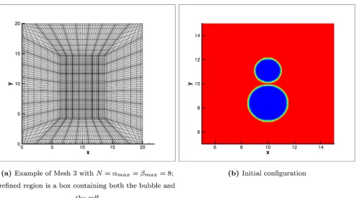
[image:13.595.42.551.54.208.2] [image:13.595.40.551.229.386.2]

Fig.12. (a)ExampleofMesh3withN=αmax=βmax=8;refinedregionisaboxcontainingboththebubbleandthecell.(b)Initialconfiguration.

to oscillate but not burst or produce a high speed jet. At these lower intensities, severalmechanisms havebeen proposed which mayenabledruguptakeintothecell(Lentacker etal., 2014).Itis possiblethat theoscillations ofthebubbleproducea poreinthe cell membrane through the exertion of fluid mechanical stresses onthecellinterfaceformedbytheassociatedmicrostreamingflow (Wu,2002).Itisalsopossiblethatthebubblewouldmigrateinto, ordirectlypushupon, thenearbycellduetothe acousticforcing (Lentacker etal., 2014). The above mechanical actions are in ad-ditiontobiologicalprocesseswheredruguptakemaybeachieved through endocytosis (the process by which cells absorb external molecules by engulfing them in their cell membrane). It is un-known which method produces the greater volume of drug de-livery intothecell,butnumericalsimulations,such asthose pre-sentedhere,mayofferimportantphysicalinsights.

Theresultspresentedpreviouslyinthisarticle,assumethatthe bubble is small in diameter in comparison to an adjacent fluid layer, which may model a large (locally flat) cell or a contami-nant layertobe removedvia microbubblecleaning.Thediameter ofcellsinthehumanbodycanvarysignificantly,ascanthe diam-eterofmicrobubbles.Forexample,typicallythediameterofan en-capsulated microbubbleused inconjunctionwithultrasound,can varybetween1₋10

μ

m(Cocketal.,2015).Therefore,thissection presents the interaction between a bubble and a full suspended cell,wherethetwohavesimilarspatialdimensions.

Itwasshownintheprevious sections,that theinteraction be-tweentherigidwallandthebubbleisdominantoverthe bubble-cellinteraction.Therefore,ourdomainischosen tobesufficiently large to negateany wall effects. Let

=[0,20]×[0,20] and as-sumethatthebubbleissituateddirectlyontopofthecellwhere the centre point between the cell and the bubble is placed in the centre of the domain. The initial configuration is illustrated in Fig.12bandtheassociatedmeshisdepictedin Fig.12abelow. The meshparameters are: N=10,

α

max=12,

β

max=12.Initially, the adjacent cell will be modelled as a Newtonian viscous drop

Table1

Dimensionalandnon-dimensionalparametersusedinthissection.

Dimensional Non-dimensional Radius Bubble Rb,0=10−6 R∗b,0=1

Cell Rc,0=1.5×10−6 R∗c,0=1.5

Density Bubble ρb,0=1 ρb∗,0=1

Fluid ρf,0=0.2 ρ∗f,0=0.2

Cell ρc,0=0.2 ρc∗,0=0.2

DynamicViscosity Bubble ηb,0=10−5 η∗b,0=0.033

Fluid ηf,0=10−4 η∗f,0=0.333

Cell ηc,0=10−3 η∗c,0=3.333

KinematicViscosity Bubble μb,0=10−5 μ∗b,0=0.033

Fluid μf,0=5×10−4 μ∗f,0=1.665

Cell μc,0=5×10−3 μ∗c,0=16.665

SpeedofSound c¯0=1500 c¯∗0=5

(Section6.1).However, inreality,cellswillexhibit viscoelastic be-haviourduetothevariousmicrostructures thatarepresentinthe cell’s interior.Therefore, we also consider a viscoelasticfluid ap-proximationoftheadjacentcellin Section6.2.

6.1. Newtonianfluid

Thedimensionalandnon-dimensionalparameters usedinthis section are given in Table 1. To calculate the non-dimensional parameters, we employ the same scaling as given earlier in Section2.1wheretheinitial bubbleradiusR=1

μ

m,initial bub-bledensity

ρ

_b,0=1kg_·m−3 _(⇒q

b,0=0) andthereferencespeed of soundV=3×102 _ms−1 _{(the speed of soundthrough the air} phase). The bubble,fluid and cell viscositiesare of the (approxi-mate)orderstypicallyfoundforair,bloodplasmaandaredblood cell’shaemoglobinsolution(see e.g. McClainetal., 2004), respec-tively. Note that the speed of sound parameter is taken to be

¯

c0=1500ms−1.

[image:14.595.50.559.51.334.2] [image:14.595.324.550.391.515.2]

132 C.F.Rowlatt,S.J.Lind/InternationalJournalofMultiphaseFlow90(2017)118–143

Fig.13. Illustrationofthecolourfunctionwithvelocitystreamlines,densitycontour,streamlinenormalandshearstressesattimet=0.1.

timest₌0_.1_,0_.2_,0_.3_,0_.5_,respectively.Incontrasttotheprevious sections,wewishtosimulateaninitialexpansionphase(thelikes ofwhich wouldbe seenwhen abubblerespondstoa ultrasound wavetrough).Thus,theinitial density(andtherefore,initial pres-sure)inside the bubble istaken to be larger than thedensity in theambient fluid so that the bubble expandsinitially (Fig. 13a). Theinitialexpansion,releasesanapproximatelysphericalpressure wave(Fig.13b), intothesurrounding fluidwhich dissipatesfairly rapidly.This pressurewave induces a highinmagnitude stream-linenormalstress atthe top ofthecell (Fig.13c). Asthe bubble expands,itpushesintothenearbycellwhichcausesaflatteningof boththecellandthebubble,whichcanclearlybeseenin Figs.14a, 15aand 16a.At latertimes,thegapbetweenthe bubbleandcell increasesslightly dueto the continuing expansion of the bubble

pushing thecell downwards.As a resultofthebubble expansion intothe nearbycell,a regionofhighpressure develops,and per-sists,atthebottomofthebubbleandtopofcellsurface(Figs.14b, 15band 16b).Thispersistenthighpressureisreflectedinthehigh normalstress region atthe cell interface (Figs. 14c, 15c and 16c) which issustained forthewhole simulation, evenas thenormal stress elsewhere begins to spread and dissipate around the cell surface.Due tothenormalstressbeingconcentrated ata specific locationinthecell,itcould havepotentiallynegativeimplications forcellfunctionality.

[image:15.595.38.553.54.560.2]

Fig.14. Illustrationofthecolourfunctionwithvelocitystreamlines,densitycontour,streamlinenormalandshearstressesattimet=0.2.

membraneofthe cell. Fig.13d illustrates thebuild upof stream-lineshearstressonthefluid-cellinterface.Thisshearstressis pro-ducedbythevelocityfieldbendingaround thefluid-cell interface as can be seen in Figs. 15a and 16a. Figs. 15d and 16d illustrate that the shear stress spreads around thefluid-cell interface from towardsthetopofthecelltothemiddle,implyingthat a cavitat-ingbubblecanhaveaglobaleffectonthecell. Leowetal.(2015), showedthatso-calledblebbing(atermusedtodescribealocal dis-tortioninthemembraneofacell)occurred,notonlyatthe sono-poration site(e.g. the site ofjet impact - inertial cavitation) but also along the membrane periphery. It was concludedthat bleb-bingattheimpactsitemaybeinvolvedinthecell’srepairprocess butnoreasonsareofferedfortheadditionalblebbingfoundalong themembranesperiphery. Leowetal.(2015)doindicatethat

non-localblebbing isquite likely, giventhat the actin cytoskeleton(a fibrousnetworkintheinteriorofacellwhichisconnectedtothe cellmembrane)isdisrupted(seee.g. Chenetal.,2014).Theresults presentedhereillustrate spreading ofboth thenormal andshear stressesalongthecellmembrane:aphenomenonpurely hydrody-namicalinnature.Thisraisesthepossibilitythatthe hydrodynam-icalspreadingofnormalandshearstressesisthekeymechanism increatingnon-localisedblebbing(andalsonon-localdisruptionof theactincytoskeletonclosetothecellmembrane),ratherthanany biochemicalcellresponse.

6.2.Viscoelasticfluid

[image:16.595.50.560.51.563.2]

134 C.F.Rowlatt,S.J.Lind/InternationalJournalofMultiphaseFlow90(2017)118–143

Fig.15. Illustrationofthecolourfunctionwithvelocitystreamlines,densitycontour,streamlinenormalandshearstressesattimet=0.3.

(Eq. (3)) can be supplemented by an additional term describing the polymeric stress contribution

τ

, where the polymeric stress satisfiesan additionalconstitutivelaw.The Oldroyd-Bviscoelastic modelisanaturalchoice duetoitssimplicityandprevioususage withinthecompressibleSEMPframework(LindandPhillips,2013). Thus, Eq.(3)becomes:

S =

η

s

1

∇

u+

∇

uT

₊

η

s

2

(

∇

·u

)

I +

τ

, (19) wherethe polymeric stress

τ

satisfies a constitutive equation of (compressible)upper-convectedMaxwell(UCM)type:

τ

+

λ

1

τ

+

(

∇

·u

)

τ

=

η

p

1

∇

u+

∇

uT

₍₂₀₎

wherethesuperscriptss andpdenote thesolventandpolymeric viscosities, respectively, and

λ

1 denotes the characteristic

relax-ation time. The symbol · denotes theupper-convectedderivative andisdefinedby

τ

= D

τ

Dt −

(

∇

u

)

τ

−

τ

(

∇

u

T

₎

₍₂₁₎

Note that when

η

s

1=

η

s2=0, the Olroyd-B model reduces to an upper-convectedMaxwell(UCM)model.Employingthesame non-dimensionalisation as that used in Section 2.1, introduces the Weissenbergnumber,

Wi:=

λ

1V

R (22)

[image:17.595.36.550.56.553.2]

Fig.16. Illustrationofthecolourfunctionwithvelocitystreamlines,densitycontour,streamlinenormalandshearstressesattimet=0.5.

Weissenberg number problem). However, no stabilitisation tech-niques are employed in thisarticle. The non-dimensional consti-tutiveequationforthepolymericstressisthengivenby

τ

+ Wi

τ

+

(

∇

·u

)

τ

=

η

p

1

∇

u+

∇

uT

₍₂₃₎

For further information regarding the viscoelastic constitutive equation givenin Eq. (20), andits equivalentlog-density formu-lation,thereaderisreferredto LindandPhillips(2013).

In this section, the non-dimensional parameters for the bub-ble,ambient(Newtonian)fluidandsolvent(Newtonian) contribu-tiontotheviscoelasticcell,arethesameasthosegivenin Table1. Thenon-dimensionalparametersforthepolymericcontributionto the viscoelastic cell are given by:

μ

_cp_,0=1 (kinematic polymeric viscosity) andWic,0=10(Weissenberg number).Givenvalues for

cell elasticityquoted in the numericalstudy of Khismatullin and Truskey(2004) (where thevalueswere takenfromexperiments), wechoosea Weissenbergnumbercloseto thelargestallowedby themethodbeforethehighWeissenbergnumericalinstability de-stroysthesolution.

[image:18.595.48.559.54.561.2]

136 C.F.Rowlatt,S.J.Lind/InternationalJournalofMultiphaseFlow90(2017)118–143

Fig.17. Illustrationofthestreamlinepolymericnormalandshearstressesattimet=0.1.

Fig.18. Illustrationofthestreamlinepolymericnormalandshearstressesattimet=0.2.

For the choice of polymeric viscosity and Weissenberg number studiedhere,themagnitudeofthenormalandshearstressesare muchsmallerin Fig.17aandbwhencomparedtotheirNewtonian equivalents(Fig.13candd).

Once again, similar to the Newtonian case, asthe bubble ex-pands, it pushes into the nearby cell which causes a flattening ofboth the cell andthe bubble(see e.g. Figs. 14a, 15a and 16a). Similarto Section 6.1, atlatertimes thegapbetweenthe bubble andcell increasesslightlyduetothecontinuingexpansion ofthe bubblepushing thecelldownwards.Asa resultofthebubble ex-pansioninto thenearby cell, a region of highpressure develops, andpersists,at thebottom of thebubble andtop ofcell surface

(Figs.14band 15b).Itcanbeseenfrom Figs.18a, 19aand 20athat thehighestmagnitudeofstreamlinenormalstressoccursinathin layerjustinsidethefluid-cellinterface.Additionally,itcanbeseen thatthenormalstressspreadsmoreevenlythroughoutthewhole cell asthesimulation progresses.Indeed, thepresence of elastic-ityresults ina more evenly distributedstress being sustainedin thecell,resemblingbehaviourthatmightbeexpectedfroma con-nectedinternalmicro-structure.

[image:19.595.38.549.57.291.2] [image:19.595.41.551.329.575.2]

Fig.19.Illustrationofthestreamlinepolymericnormalandshearstressesattimet=0.3.

Fig.20. Illustrationofthestreamlinepolymericnormalandshearstressesattimet=0.5.

illustrated in Fig.17b.Although,initially verysmallin magnitude O

(

10−3

)

_, the magnitude increases as the simulation progresses. Also note that similar to the previous Newtonian case, Figs. 18b, 19b and 20b illustrate that the shear stress spreads around the fluid-cellinterfaceasthesimulationsprogresses.However,wenote thatthestressismuchthinnerandtherefore,muchmore concen-tratedon(orcloseto)thefluid-cellinterface.Onceagain,the non-localaction of(polymeric)normalandshear stressessupportthe possibilitythatthenon-localisedblebbingphenomena(Leowetal., 2015)ishydrodynamicalinorigin.

7. Conclusions and future work

[image:20.595.50.561.57.292.2] [image:20.595.45.559.330.574.2]