A high-order upwind control-volume method based on
integrated RBFs for fluid-flow problems
N. Mai-Duy
∗and T. Tran-Cong
Computational Engineering and Science Research Centre
Faculty of Engineering and Surveying
University of Southern Queensland, Toowoomba, QLD 4350, Australia
Short title: Integrated-RBF based Upwind Control Volume Method
Submitted to
International Journal for Numerical Methods in Fluids
,
15-Jun-2010; revised, 28-Sep-2010
Summary This paper is concerned with the development of a high-order upwind con-servative discretisation method for the simulation of flows of a Newtonian fluid in two dimensions. The fluid-flow domain is discretised using a Cartesian grid from which non-overlapping rectangular control-volumes are formed. Line integrals arising from the inte-gration of the diffusion and convection terms over control volumes are evaluated using the middle-point rule. One-dimensional integrated radial basis function schemes using the multiquadric basis function are employed to represent the variations of the field variables along the grid lines. The convection term is effectively treated using an upwind scheme with the deferred-correction strategy. Several highly-nonlinear test problems governed by the Burgers and the Navier-Stokes equations are simulated, which show that the proposed technique is stable, accurate and converges well.
Key words: integrated RBF, Cartesian grid, control volume, upwind scheme, deferred correction technique, high-order approximation
1
Introduction
algebraic system. Recognising these, various schemes that take the influence of the upwind information of the flow into account, e.g. the upwind differencing [3], power-law [4] and QUICK [5] schemes, have been developed.
The original upwind (upwind-difference/upstream-difference/donor-cell) scheme, which simply replaces the face value of the convected property with its value at the grid point on the upwind side of the face, is able to ensure positive coefficients. However, this scheme is only first-order accurate and causes a false diffusion/artificial viscosity. The power-law scheme, which can also guarantee the positivity of all coefficients, has a blended first/second order accuracy. When the local grid Peclet numbers exceed a value of 6, this scheme switches to the first-order upwinding scheme and the physical diffusion is therefore suppressed [6]. Such formulations do not work well for the cases where the flow streamlines are not closely aligned with the grid lines. On the other hand, the QUICK scheme employs a quadratic interpolation at three consecutive nodes (the two nodes located on either side of the face and the adjacent node on the upstream side) to represent the convective term. The QUICK scheme results in a better accuracy and avoids the stability problems of central differencing. Unlike upwind differencing, this quadratic interpolation scheme may produce negative coefficients and as a result its coefficient matrix may not be diagonally dominant.
Radial basis functions (RBFs) have been extensively used in solving differential problems (e.g. [9]). These approximators are able to work well (i.e. providing fast convergence) with gridded and scattered data points especially for regular node arrangements. The RBF approximations can be constructed through differentiation (e.g. [10]) or integration (e.g. [11,12,13]). The latter has the ability to avoid the reduction in convergence rate caused by differentiation and to provide an effective way of implementing derivative boundary values. Integrated RBFs (IRBFs) were successfully introduced into the CV formulation [14]. All of our previous IRBF works treated the diffusion and convection terms implicitly and explicitly, respectively. In this study, the diffusion term is approximated using global and local one-dimensional IRBF schemes, namely Scheme 1 and Scheme 2, respectively. The convection term is effectively treated here by a high-order upwind scheme incorporating global 1D-IRBFs with the deferred-correction strategy. The proposed schemes achieve both good accuracy and stability properties.
The remainder of the paper is organised as follows. Brief reviews of the CV formulation and 1D-IRBFs are given in Sections 2 and 3, respectively. Section 4 describes the two proposed discretisation schemes. In Section 5, two examples - heat transfer and fluid flow - are presented to demonstrate the attractiveness of the present implementation. Section 6 concludes the paper.
2
Control-volume formulation
Consider the following convection-diffusion equation
∂
interest.
The above equation presents the conservation principle for φover an infinitesimal control volume (i.e. there is a balance between the rate of change of φ, the convective flux rate, the diffusion flux rate and the generation rate). By directly integrating (1) over a control volume of the grid point P, ΩP, the following equation is obtained
Z
ΩP
∂
∂t(ρφ) +∇.(ρvφb )− ∇.(κ∇φ) +R
dΩP = 0, (2)
which possesses the conservative property for φ for a finite control volume.
Applying the Gauss divergence theorem to (2) results in
∂ ∂t
Z
ΩP
(ρφ)dΩP +
Z
ΓP
(ρbvφ).bndΓP −
Z
ΓP
(κ∇φ).bndΓP +
Z
ΩP
RdΩP = 0, (3)
where ΓP is the boundary of ΩP; nb the unit outward vector normal to ΓP and dΓP a
differential element of ΓP. The governing differential equation (1) is thus transformed
into a CV form (2)/(3). It is noted that no approximation is made at this stage.
3
One-dimensional IRBF scheme
The basic idea of the integral RBF scheme is to decompose the highest-order derivatives of φ in a given differential equation (e.g. second-order derivatives for the convection-diffusion equation (1)) into RBFs. Consider a univariate function φ(x). The present 1D-IRBF scheme starts with
d2φ(x)
dx2 =
N
X
i=1
where N is the number of RBFs, {wi}Ni=1 the set of network weights, and nIi(2)(x)oN
i=1
the set of RBFs. Expressions for the first-order derivative and function itself are then obtained through integration
dφ(x)
dx = N
X
i=1
wiIi(1)(x) +c1, (5)
φ(x) =
N
X
i=1
wiIi(0)(x) +c1x+c2, (6)
where Ii(1)(x) =
R
Ii(2)(x)dx, I
(0)
i (x) =
R
Ii(1)(x)dx; and (c1, c2) are the constants of
inte-gration. It is noted that the superscript (.) is used to indicate the derivative order of
φ. In the present work, 1D-IRBFs are implemented with the multiquadric (MQ) function and one has
Ii(2)(x) =
q
(x−ci)2+a2
i, (7)
Ii(1)(x) =
(x−ci) 2 A+
a2
i
2B, (8)
Ii(0)(x) =
−a2
i
3 +
(x−ci)2
6
A+a
2
i(x−ci)
2 B, (9)
whereciandaiare the centre and the width of theith MQ, respectively;A =p(x−ci)2+a2
i;
and B = ln(x−ci) +p(x−ci)2+a2
i
.
Evaluation of (4)-(6) at a set of collocation points {xi}Ni=1 (also a set of the MQ centres here, {xi}Ni=1 ≡ {ci}Ni=1) leads to
d
d2φ
dx2 =Ib (2)
b
α, (10)
c
dφ dx =Ib
(1)
b
α, (11)
b
where
b
I(2) =
I1(2)(x1), I2(2)(x1), · · · , IN(2)(x1), 0, 0
I1(2)(x2), I2(2)(x2), · · · , IN(2)(x2), 0, 0
... ... . .. ... ... ...
I1(2)(xN), I2(2)(xN), · · · , IN(2)(xN), 0, 0
, b
I(1) =
I1(1)(x1), I2(1)(x1), · · · , IN(1)(x1), 1, 0
I1(1)(x2), I2(1)(x2), · · · , IN(1)(x2), 1, 0
... ... . .. ... ... ...
I1(1)(xN), I2(1)(xN), · · · , IN(1)(xN), 1, 0
, b
I(0) =
I1(0)(x1), I2(0)(x1), · · · , IN(0)(x1), x1, 1
I1(0)(x2), I2(0)(x2), · · · , IN(0)(x2), x2, 1
... ... . .. ... ... ...
I1(0)(xN), I2(0)(xN), · · · , IN(0)(xN), xN, 1
; b
α= (w1, w2,· · ·, wN, c1, c2)T ;
and
d
dkφ dxk =
dkφ
1
dxk , dkφ
2
dxk ,· · · , dkφN
dxk
T
, k= (1,2),
b
φ= (φ1, φ2,· · · , φN)T ,
in which dkφi/dxk =dkφ(xi)/dxk and φi =φ(xi) with i= (1,2,· · · , N).
conversion of the RBF weight space into the physical space
b
φ
b
e
=
Ib
(0)
b
K
bα=Cbα,b (13)
where be = (e1, e2)T is a vector representing extra information (e.g. normal derivatives
and differential equations at the boundaries); eb= Kbαb; φb, Ib(0) and αb defined as before;
and Cbthe conversion matrix. It can be seen from (13) that the approximate solution φ is collocated at the whole set of centres. Solving (13) for αb yields
b
α=Cb−1
φb
b
e
, (14)
whereCb−1 is the inverse or pseudo-inverse ofCb, depending on its dimensions. The cost for
Substitution of (14) into (4)-(6) leads to
φ(x) =I1(0)(x), I2(0)(x),· · ·Cb−1
b φ b e
, (15)
∂φ(x)
∂x =
I1(1)(x), I2(1)(x),· · ·Cb−1
φb
b
e
, (16)
∂2φ(x)
∂x2 =
I1(p)(x), I2(p)(x),· · ·Cb−1
b φ b e
. (17)
They can be rewritten in the form
φ(x) =
N
X
i=1
ϕi(x)φi+ϕN+1(x)e1+ϕN+2(x)e2, (18)
∂φ(x)
∂x = N
X
i=1
dϕi(x)
dx φi+
dϕN+1(x)
dx e1+
dϕN+2(x)
dx e2, (19) ∂2φ(x)
∂x2 =
N
X
i=1
d2ϕi(x)
dx2 φi+
d2ϕN +1(x)
dx2 e1+
d2ϕN +2(x)
dx2 e2, (20)
where {ϕi(x)}Ni=1+2 is the set of basis functions in the physical space.
4
Proposed method
the first-order backward Euler implicit formula. Equation (3) thus becomes
ρP∆AP
∆t φP −φ
0
P
+ [(ρuφ)e∆y−(ρuφ)w∆y+ (ρvφ)n∆x−(ρvφ)s∆x]−
κ∂φ ∂x
e
∆y−
κ∂φ ∂x
w
∆y+
κ∂φ ∂y
n
∆x−
κ∂φ ∂y s ∆x
+RP∆AP = 0, (21)
where the superscript 0 represents the value obtained from the previous time level; the subscripts e, w, nands denote the values of the property at the middle points of the east, west, north and south faces of a control volume; ∆AP the area of ΩP; RP the value of R
at node P; and uand v the x− and y−component of bv.
It can be seen that expressions for computing the interface values on thex− and y−grid lines have similar forms. Thus, in the following, details will be given for an x−grid line only.
4.1
Diffusion approximations
4.1.1 Scheme 1
Using (19), the face value is computed as
∂φ ∂x e = Nx X i=1
dϕi(xe)
dx φi+
dϕNx+1(xe)
dx e1 +
dϕNx+2(xe)
dx e2, (22)
∂φ ∂x w = Nx X i=1
dϕi(xw)
dx φi+
dϕNx+1(xw)
dx e1+
dϕNx+2(xw)
dx e2, (23)
where Nx is the total number of nodes on the x−grid line. These approximations are global and hence guarantee that the flux is continuous across the interface between any two adjoining control volumes (the first CV rule).
4.1.2 Scheme 2
The face value is evaluated as
∂φ ∂x e = 3 X i=1
dϕi(xe)
dx φi+
dϕ4(xe)
dx e1 +
dϕ5(xe)
dx e2, (24)
∂φ ∂x w = 3 X i=1
dϕi(xw)
dx φi+
dϕ4(xw)
dx e1+
dϕ5(xw)
dx e2. (25)
These approximations are local and constructed on overlapping regions that are defined between the west and east grid points of node P. The resultant matrix of Scheme 2 is much more sparse than that of Scheme 1.
4.2
Convection approximations
stability of a numerical scheme. From the physical point of view, convection represents the flow from upstream to downstream. One can thus expect that the upstream nodal value of
φ, denoted by φU, would make quite an impact on the value ofφat the interface, denoted by φf. It is noted that the subscript f can be e or w. We treat the convection term here by an upwind scheme incorporating global 1D-IRBFs with the deferred-correction strategy
φf =φU + ∆φf, (26)
where
∆φf =
U−1
X
i=1
ϕi(xf)φ0i + (ϕU(xf)−1)φ0U + Nx
X
i=U+1
ϕi(xf)φ0i +ϕNx+1(xf)e1+ϕNx+2(xf)e2,
in which {φ0
i} Nx
i=1 are the nodal values of φ obtained from the previous time level. The
streamwise correction term ∆φf is therefore known at the current time level. Expression (26) ensures diagonal dominance for the resultant system of algebraic equations and ap-proximate solutions can therefore evolve in a stable manner (i.e. solution is physically meaningful at all times). At convergence, the accuracy ofφf is determined by the global 1D-IRBF scheme.
It can be seen that Scheme 2 has the same structure of the system matrix (i.e. the tridiagonal and pentadiagonal forms for 1D and 2D problems, respectively) as the standard CV techniques.
5
Numerical examples
The performance of the proposed discretisation schemes, i.e. Scheme 1 and Scheme 2, is studied through the solution of the Burgers and Navier-Stokes equations. The latter is taken in the stream-function and vorticity formulation. The grid size, h, is chosen as the MQ width. All PDEs under consideration here are subject to Dirichlet boundary conditions. The extra information vectorbe in (13) is set to null for solving the PDEs and to derivative boundary values of the stream function for deriving computational boundary conditions for the vorticity. For comparison purposes, the standard CV techniques, where the diffusion term is discretised using central differences, are also employed here. If the convection term is treated using the original upwind version, we name it an UW-CD technique. If the convection term is treated using the central-difference formulation, it is then called an CD-CD technique. Scheme 2 can somehow serve as a tool to measure the relative performance of the upwind scheme based on 1D-IRBFs to those based on polynomials. Time-dependent equations are solved by the time-marching approach. A computed solution at a lower Reynolds number is used as the initial condition. For the special case of Stokes equations, the flow starts from rest. We utilise banded and iterative solvers to solve the algebraic equation sets.
5.1
Example 1
Consider the following non-linear Burgers equation
dφ dt +φ
dφ dx =ε
d2φ
on the domainxA≤x≤xB with Dirichlet boundary conditions, whereεis a given value. We consider steady flows, for which analytical solutions are given by
φ(x) = −tanhx 2ε
. (28)
Calculations are carried out on uniformly-distributed nodes.
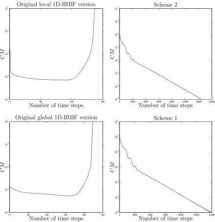
To investigate the convergence behaviour of the two present discretisation schemes, a global 1D-IRBF-based CV technique, where the diffusion and convection terms are re-spectively treated implicitly and explicitly, is also considered. This technique is referred to as the original IRBF version. As discussed earlier, the original IRBF version and Scheme 1 will give the same accuracy when the solutions are converged. For Scheme 2, the coefficient matrix is tridiagonal. When the discrete relative norm of φ between two successive time levels,tol, is less than 10−7, the flow is considered to reach a steady state.
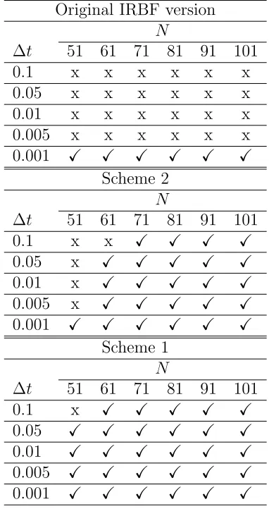
Different time steps, namely 0.1, 0.05, 0.01, 0.005 and 0.001, are employed. Results are presented in Table 1, indicating that much larger time steps can be used with the present schemes. Scheme 1 works better than Scheme 2.
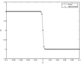
To assess accuracy of the two present schemes, we employ the UW-CD technique. The error is measured using the discrete relative norm of φ, denoted by Ne(φ), at a test set of 501 uniformly distributed points. Table 2 shows that the present schemes especially Scheme 1 significantly outperform the UW-CD technique regarding accuracy, i.e. up to two orders of magnitude for Scheme 1. In addition, Scheme 1 gives a very fast convergence, i.e. up toO(h7.85), as shown in Table 3. A computed solution by Scheme 1 together with
5.2
Example 2
Recirculating laminar incompressible flows of a Newtonian/non-Newtonian fluid in en-closed cavities have received a great deal of attention in fluid mechanics community as they can produce interesting flow features at different Reynolds/Weissenberg numbers. Examples of this type include lid-driven flows in square and triangular cavities. The top wall (lid) slides at a constant velocity. For such problems, at the two top corners, the velocity is discontinuous and the stress is unbounded, which poses great challenges for numerical simulation. This study is concerned with a Newtonian fluid and cavities of square and equilateral triangular shapes. The governing equations are employed in the form of the stream function (ψ) and vorticity (ω)
ω=∇.(∇ψ), (29)
∂ω
∂t +∇.(bvω) =
1
Re∇.(∇ω), (30)
where bv = (u, v)T = (∂ψ/∂y,−∂ψ/∂x)T and Re is the Reynolds number.
Boundary nodes are generated here using grid lines that pass through interior grid nodes. As a result, the set of RBF centres/collocation-points does not include the two top corners (the triangular cavity) and the four corners (the square cavity). By this simple treatment, it can be seen that infinite values of the vorticity do not enter the discrete system. 1D-IRBFs are employed on each grid line to represent the field variable and its derivatives in solving (29) and (30).
5.2.1 Square cavity
7704 to 8031. In this study, the time-dependent Navier-Stokes equations are solved for a wide range ofRe, namely (100, 1000, 3200, 5000, 7500), where uniform grids are employed. Results obtained are compared with the benchmark solutions provided by Ghia et al. [8] and Botella and Peyret [16]. The former was obtained using a multi-grid based finite-difference method with fine grids. For the latter, Chebyshev polynomials and analytic formulations were employed to handle the regular and singular parts of the solution and the benchmark results were given forRe= 100 and Re= 1000.
Using (20), for the two vertical walls, computational boundary conditions for the vorticity are obtained as follows
ω1 =
∂2ψ 1
∂x2 =
Nx
X
i=1
d2ϕi(x 1)
dx2 ψi+
d2ϕN
x+1(x1)
dx2
∂ψ1
∂x + d2ϕN
x+2(x1)
dx2
∂ψNx
∂x , (31)
ωNx =
∂2ψN
x
∂x2 =
Nx
X
i=1
d2ϕi(xN
x)
dx2 ψi+
d2ϕN
x+1(xNx)
dx2
∂ψ1
∂x + d2ϕN
x+2(xNx)
dx2
∂ψNx
∂x . (32)
By means of point collocation and integration constants, derivative boundary values are thus incorporated into the 1D-IRBF approximations in an exact manner. They are forced to be satisfied exactly. Moreover, all grid points on the associated grid lines are used to compute ω1 and ωNx. As a result, the present treatment possesses some global ap-proximation properties. Expressions for ω at the two horizontal walls are obtained in an analogous manner. They are used for Scheme 1 and Scheme 2 and also for the present UW-CD and CD-CD techniques.
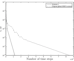
steps can thus be used with the present schemes, making the convergence much faster as shown in Figure 3.
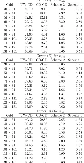
Results concerning the extreme values of the velocity profiles on the vertical and horizontal centreline for Re = 1000 are presented in Table 4. Both Scheme 1 and Scheme 2 produce results that are much closer to the spectral benchmark results than the UW-CD and CD-CD techniques. It can be seen that the UW-CD-CD technique suffers from serious inaccuracy. Again, Scheme 1 is more accurate than Scheme 2.
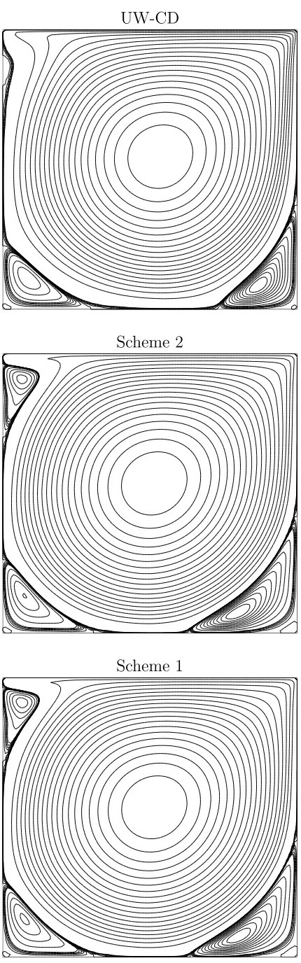
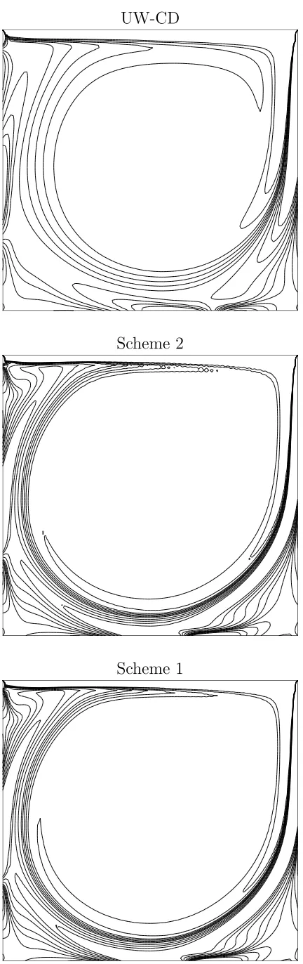
AtRe = 5000, the flow is simulated with the present schemes and the UW-CD technique. Contour plots for the stream function and the vorticity are shown in Figures 4 and 5, respectively. It can be seen that a secondary vortex in the region close to the top left corner by the UW-CD technique has a much smaller size than those produced by the present schemes. Figure 6 shows the velocity profiles on the vertical and horizontal centrelines, where results by Ghia et al. [8] are also included for comparison purposes. It can be seen that the UW-CD technique produces lower velocity extreme values than the present schemes. The present results are in very good agreement with those produced by Ghia et al. [8]. For the vorticity field, Scheme 1 produces a smoother solution than Scheme 2.
AtRe= 7500, simulations are carried out with Scheme 1 and Scheme 2. A uniform grid of 131×131 is found to be sufficient for obtaining accurate results including the vorticity field as shown in Figure 7.
5.2.2 Triangular cavity
reference length and velocity are presently chosen asL=Q/3 andU = 1 (the velocity of the lid), respectively. It is noted that this problem was numerically studied by different techniques, including the finite-difference method (e.g. [18]) and the finite-element method (e.g. [19]). In early numerical studies, e.g. [18,20], finite differences were constructed on a transformed geometry and the flows were considered for Re ≤ 500 only. Later on, solutions for higher Re numbers were achieved by means of, for example, the so-called computational boundary method in which the computational region under consideration is one-grid inside the physical domain [21] and the flow-condition-based interpolation [19].
At the lid, the imposition of boundary conditions for ω is similar to that used in the square cavity flow. At the left and right walls, analytic formulae for computing the vorticity boundary condition on a non-rectangular boundary [22] are utilised here:
ωb =
1 +
tx ty
∂2ψb
∂x2 , (33)
for ax−grid line, and
ωb =
1 +
ty tx
∂2ψb
∂y2 , (34)
for a y−grid line. In (33) and (34), tx and ty are the x− and y−components of the unit vector tangential to the boundary. The two formulae (33) and (34) require the approximations be conducted in one direction only. No exterior/fictitious points are used here.
Its computer codes are run on a PC with the total physical memory of 1024 MB. To investigate the upwinding effects, an original local 1D-IRBF version is also employed. This version is similar to Scheme 2 except that the convection term is treated explicitly. As shown in Figure 9, a much larger time step can be used with Scheme 2 that converges much faster than the original local 1D-IRBF version.
Figures 10 and 11 present contour plots of the stream-function and vorticity fields, which look reasonable when compared with those available in the literature (e.g. [18,19]).
Figure 12 presents variations of the x component of the velocity vector on the vertical centreline x = 0 and the y component of velocity on the horizontal line y = 2. Results obtained in [19] are also included for comparison purposes. It can be seen that the velocity profiles using Grid 1 are almost identical to those using Grid 2. The present results agree well with those by the flow-conditioned-based interpolation FEM for all values ofRe.
5.3
Discussion
CV method. It is noted that the value 10000 is obtained through extrapolation. For Scheme 1, the CPU time per iteration is approximately zero. For the standard CV method, at 4000 nodes (not 10000 nodes), the CPU time per iteration is already up to 0.359s. The computer codes are written using MATLAB and run on a Dell X86-based PC (Intel 2992 Mhz). In this regard (accuracy), the proposed method can be more efficient than the standard CV method. In addition, the employment of upwinding with 1D-IRBFs and deferred correction maintains the numerical stability or boundedness (first-order upwinding) and, at the same time, ensures high-order accuracy (1D-IRBFs).
6
Conclusions
This paper reports a new control-volume method, based on Cartesian grids and global/local 1D-IRBFs, for fluid-flow problems. A high-order upwind treatment with the deferred cor-rection strategy using 1D-IRBFs for the convection term is implemented to enhance the stability property to the evolving solutions. The present schemes are able to produce converging solutions of high levels of accuracy at high values of the Reynolds number for both rectangular and non-rectangular fluid-flow domains.
Acknowledgement
This work is supported by the Australian Research Council. We would like to thank the referees for their helpful comments.
2. Huilgol RR, Phan-Thien N. Fluid Mechanics of Viscoelasticity. Elsevier: Amster-dam, 1997.
3. Gentry RA, Martin RE, Daly BJ. An Eulerian differencing method for unsteady compressible flow problems. Journal of Computational Physics 1966; 1(1): 87-118.
4. Patankar SV. A calculation procedure for two-dimensional elliptic situations. Nu-merical Heat Transfer, Part B 1981; 4(4): 409-425.
5. Leonard BP. A stable and accurate convective modelling procedure based on quadratic upstream interpolation. Computer Methods in Applied Mechanics and Engineering 1979; 19(1): 59-98.
6. Leonard BP, Mokhtari S. Beyond first-order upwinding: The ultra-sharp alternative for non-oscillatory steady-state simulation of convection. International Journal for Numerical Methods in Engineering 1990; 30(4): 729-766.
7. Khosla PK, Rubin SG. A diagonally dominant second-order accurate implicit scheme. Computers & Fluids 1974; 2(2): 207-209.
8. Ghia U, Ghia KN, Shin CT. High-Re solutions for incompressible flow using the Navier-Stokes equations and a multigrid method. Journal of Computational Physics 1982; 48: 387-411.
9. Fasshauer GE. Meshfree Approximation Methods With Matlab (Interdisciplinary Mathematical Sciences - Vol. 6). World Scientific Publisher: Singapore, 2007.
10. Kansa EJ. Multiquadrics- A scattered data approximation scheme with applications to computational fluid-dynamics-II. Solutions to parabolic, hyperbolic and elliptic partial differential equations. Computers and Mathematics with Applications 1990;
19(8/9): 147-161.
12. Mai-Duy N, Tanner RI. Solving high order partial differential equations with radial basis function networks. International Journal for Numerical Methods in Engineer-ing 2005;63: 1636-1654.
13. Mai-Duy N, Tran-Cong T. Solving biharmonic problems with scattered-point dis-cretisation using indirect radial-basis-function networks. Engineering Analysis with Boundary Elements 2006; 30: 77-87.
14. Mai-Duy N, Tran-Cong T. A control volume technique based on integrated RBFNs for the convection-diffusion equation. Numerical Methods for Partial Differential Equations 2010; 26(2): 426-447.
15. Boppana VBL, Gajjar JSB. Global flow instability in a lid-driven cavity. Interna-tional Journal for Numerical Methods in Fluids 2010;62(8): 827-853.
16. Botella O, Peyret R. Benchmark spectral results on the lid-driven cavity flow. Com-puters & Fluids1998; 27(4): 421-433.
17. Jyotsna R, Vanka SP. Multigrid calculation of steady, viscous flow in a triangular cavity. Journal of Computational Physics 1995; 122(1): 107-117.
18. Ribbens CJ, Watson LT, Wang C-Y. Steady viscous flow in a triangular cavity. Journal of Computational Physics 1994; 112(1): 173-181.
19. Kohno H, Bathe K-J. A flow-condition-based interpolation finite element procedure for triangular grids. International Journal for Numerical Methods in Fluids 2006;
51(6): 673-699.
Table 1: Burgers equation, xA = −0.1, xB = 0.1, ε = 10−3, tol = 10−7, φ(x,0) = (φB−
φA)/(xB−xA)x, time-marching solver: convergence study for the original IRBF version and the two present schemes. Converging and diverging solutions are denoted as X and
x, respectively.
Original IRBF version
N
∆t 51 61 71 81 91 101
0.1 x x x x x x
0.05 x x x x x x
0.01 x x x x x x
0.005 x x x x x x 0.001 X X X X X X
Scheme 2
N
∆t 51 61 71 81 91 101
0.1 x x X X X X
0.05 x X X X X X
0.01 x X X X X X
0.005 x X X X X X
0.001 X X X X X X
Scheme 1
N
∆t 51 61 71 81 91 101
0.1 x X X X X X
0.05 X X X X X X
0.01 X X X X X X
0.005 X X X X X X
Table 2: Burgers equation, xA = −0.1, xB = 0.1, ε = 10−3, tol = 10−7, φ(x,0) = (φB−
φA)/(xB−xA)x,∆t = 0.001: accuracy by the UW-CD method and by the present schemes. It is noted that the error Ne(φ) is computed at a test set of 501 uniformly distributed points.
Ne(φ)
Table 3: Burgers equation, xA = −0.1, xB = 0.1, ε = 10−3, tol = 10−7, φ(x,0) = (φB−
φA)/(xB−xA)x,∆t = 0.005: convergence rates by Scheme 1.
h Convergence rates
4.00e-3
-3.33e-3 O(h2.54)
2.85e-3 O(h2.97)
2.50e-3 O(h3.40)
2.22e-3 O(h3.84)
2.00e-3 O(h4.29)
1.81e-3 O(h4.73)
1.66e-3 O(h5.17)
1.53e-3 O(h5.61)
1.42e-3 O(h6.03)
1.33e-3 O(h6.45)
1.25e-3 O(h6.84)
1.17e-3 O(h7.21)
1.11e-3 O(h7.55)
Table 4: Square-cavity flow,Re= 1000: Percentage errors relative to the spectral bench-mark results for the extreme values of the velocity profiles on the centrelines.
Errors (%) for umin
Grid UW-CD CD-CD Scheme 2 Scheme 1 31×31 46.10 29.19 12.85 11.86 41×41 38.17 18.13 7.92 6.50 51×51 32.92 12.11 5.34 4.09 61×61 29.12 8.63 3.80 2.80 71×71 26.21 6.46 2.81 2.03 81×81 23.88 5.02 2.14 1.54 91×91 21.95 4.01 1.66 1.19 101×101 20.33 3.28 1.32 0.96 111×111 18.94 2.73 1.05 0.78 121×121 17.74 2.31 0.84 0.65 131×131 16.69 1.98 0.65 0.55
Errors (%) for vmax
Grid UW-CD CD-CD Scheme 2 Scheme 1 31×31 48.01 29.98 13.05 11.91 41×41 39.71 18.45 8.02 6.55 51×51 34.43 12.32 5.40 4.13 61×61 30.62 8.79 3.84 2.83 71×71 27.68 6.58 2.83 2.05 81×81 25.31 5.12 2.14 1.56 91×91 23.34 4.09 1.66 1.21 101×101 21.67 3.35 1.31 0.97 111×111 20.23 2.79 1.04 0.79 121×121 18.98 2.36 0.82 0.66 131×131 17.89 2.02 0.62 0.56
Errors (%) for vmin
−0.1 −0.08 −0.06 −0.04 −0.02 0 0.02 0.04 0.06 0.08 0.1 −1.5
−1 −0.5 0 0.5 1 1.5
Exact Approximate
x
[image:28.595.157.468.87.340.2]φ
Figure 1: Burgers equation, xA = −0.1, xB = 0.1, ε = 10−3, tol = 10−7, φ(x,0) =
0 50 100 150 10−4
10−3 10−2 10−1
100 Original local 1D-IRBF version
Number of time steps
C
M
0 2000 4000 6000 8000 10000 12000 14000 10−8
10−7 10−6 10−5 10−4 10−3 10−2
10−1 Scheme 2
Number of time steps
C
M
0 50 100 150 200 250 10−4
10−3 10−2 10−1
100 Original global 1D-IRBF version
Number of time steps
C
M
0 2000 4000 6000 8000 10000 12000 10−8
10−7 10−6 10−5 10−4 10−3
10−2 Scheme 1
Number of time steps
C
[image:29.595.91.530.55.509.2]M
0 1 2 3 4 5 6 7 8 9
x 104 10−8
10−7 10−6 10−5 10−4 10−3 10−2
Scheme 1
Original global IRBFN version
Number of time steps
C
[image:30.595.157.466.88.343.2]M
UW-CD
Scheme 2
[image:31.595.204.419.52.740.2]UW-CD
Scheme 2
[image:32.595.204.420.52.738.2]−0.50 0 0.5 1 0.1
0.2 0.3 0.4 0.5 0.6 0.7 0.8 0.9 1
Ghia et al. (1982)
UW−CD
Scheme 2
Scheme 1
u
0 0.1 0.2 0.3 0.4 0.5 0.6 0.7 0.8 0.9 1 −0.8
−0.6 −0.4 −0.2 0 0.2 0.4 0.6
Ghia et al. (1982)
UW−CD
Scheme 2
Scheme 1
[image:33.595.205.417.56.507.2]v
ψ, Scheme 1 ω, Scheme 1
−0.50 0 0.5 1
0.1 0.2 0.3 0.4 0.5 0.6 0.7 0.8 0.9 1
Ghia et al. (1982)
Scheme 2
Scheme 1
u
0 0.1 0.2 0.3 0.4 0.5 0.6 0.7 0.8 0.9 1 −0.8
−0.6 −0.4 −0.2 0 0.2 0.4 0.6
Ghia et al. (1982)
Scheme 2
Scheme 1
[image:34.595.94.533.54.518.2]v
x y
(0,0)
(P, Q) (−P, Q)
[image:35.595.141.472.87.387.2](ψ = 0, ∂ψ/∂n= 0) (ψ = 0, ∂ψ/∂n= 0) (ψ = 0, ∂ψ/∂n= 1)
0 2 4 6 8 10 12 14 16 18
x 104 10−8
10−7 10−6 10−5 10−4 10−3 10−2
Scheme 2
Original local IRBFN version
Number of time steps
C
[image:36.595.157.466.87.340.2]M
Re= 500, Grid 1 Re = 1000, Grid 1
[image:37.595.94.532.58.511.2]Re = 1500, Grid 2 Re = 2000, Grid 2
Re= 500, Grid 1 Re = 1000, Grid 1
[image:38.595.94.531.53.514.2]Re = 1500, Grid 2 Re = 2000, Grid 2
−1.50 −1 −0.5 0 0.5 1 1.5 0.5
1 1.5 2 2.5 3
Kohno and Bathe, 2006
Grid 1
Grid 2
Re= 100
−1.50 −1 −0.5 0 0.5 1 1.5
0.5 1 1.5 2 2.5 3
Kohno and Bathe, 2006
Grid 1
Grid 2
Re= 500
−1.50 −1 −0.5 0 0.5 1 1.5
0.5 1 1.5 2 2.5 3
Kohno and Bathe, 2006
Grid 1
Grid 2
[image:39.595.203.419.59.715.2]Re = 1000