Almost sure exponential stability of the Euler–Maruyama approximations for stochastic functional differential equations

Almost sure exponential stability of

the Euler–Maruyama approximations for

stochastic functional differential equations

Fuke Wu, Xuerong Mao and Peter E. Kloeden

Abstract.By the continuous and discrete nonnegative semimartingale convergence theo-rems, this paper investigates conditions under which the Euler–Maruyama (EM) approxi-mations of stochastic functional differential equations (SFDEs) can share the almost sure exponential stability of the exact solution. Moreover, for sufficiently small stepsize, the de-cay rate as measured by the Lyapunov exponent can be reproduced arbitrarily accurately. Keywords.Stochastic functional differential equations (SFDEs), nonnegative semimar-tingale convergence theorem, almost sure stability, EM method.

2010 Mathematics Subject Classification.60H10, 65L20.

1

Introduction

Stochastic differential equations (SDEs) and their stability have been used with great success in a variety of applications areas, including biology, epidemiology, mechanics, neural networks, economics, finance and so on. Most SDEs arising in practice are nonlinear and cannot be solved explicitly, so stability analysis of nu-merical methods for SDEs has recently received a great deal of attention. Due to the stochastic nature, the stability concepts of numerical schemes for SDEs in-clude, for example, moment stability, almost sure stability and stability in distribu-tion. There is an extensive literature concerned with the moment stability, for ex-ample, [5, 6, 8–10, 24, 29] for SDEs and [3, 20] for stochastic differential equations (SDDEs). Regarding the almost sure stability of numerical methods for SDEs, it was shown, by using the Chebyshev inequality and the Borel–Cantelli lemma, that the moment exponential stability implies almost sure exponential stability under certain conditions (for example, see [9, 24]). Higham and his coauthors ([8, 9])

rectly studied the numerical sequence and obtained almost sure stability by the strong law of large numbers. Now there is little result to examine stability in dis-tribution of numerical methods although this stability is also important. The only work can be seen in [4] and [30].

By the technique based on the continuous semimartingale convergence theorem (cf. [11,14]), Mao developed in his serial papers (see e.g. [15–18,32]) the stochas-tic versions of the LaSalle theorem, from which follows the almost sure asymptostochas-tic stability of SDEs, including SDDEs and SFDEs. On the other hand, by the discrete semimartingale convergence theorem (cf. [26,33]), [25–27] investigated the stabil-ity of stochastic difference equations and [31] examined almost sure stabilstabil-ity of the stochastic theta methods of linear SDEs. Noting that there are similar expressions for the continuous and discrete semimartingale convergence theorems, [26] ob-tained the sufficient conditions for almost surely asymptotic stability of both exact and numerical solutions of linear stochastic differential equations. Then Wu et al. [35] examined conditions under which the numerical solutions of SDDEs may share the almost sure stability of exact solutions for nonlinear SDDEs.

However, so far, little is as yet known about the stability of numerical solutions for SFDEs although there are lots of such results for the exact solutions of SFDFs (for example, [14, 17, 23, 32]). The main aim of this paper is to extend the results in [26, 35] to SFDEs and examine conditions under which the numerical solutions of SFDEs may reproduce the almost sure stability of the exact solutions. Consider then-dimensional SFDE

dx.t /Df .xt; t /dtCg.xt; t /dw.t /; t 0; (1.1) with initial datax0 D2CFb0.Œ ; 0I

Rn_{/, namely, is a bounded,}F₀ -measur-ableC.Œ ; 0IRn_{/-valued random process defined onŒ ; 0, where}

xt DWxt. /D ¹x.t C /W 0º 2C.Œ ; 0IRn/;

f; g W C.Œ ; 0R_CIRn_/R_{C !} Rn _{are Borel measurable,w.t /is a scalar} Brownian motion. For the purpose of stability, we assumef .0; t / Dg.0; t /D0. This shows that (1.1) admits a trivial solution. As a standing hypothesis, we shall impose the following local Lipschitz condition on coefficientsf andg:

Assumption 1.1.For eachk D 1; 2; : : :, there isck > 0such that for any maps

'; 2C.Œ ; 0IRn_{/and allt 0,}

jf .'; t / f .; t /j _ jg.'; t / g.; t /j ckk' k;

Let the stepsize 4be a fraction of the delay, namely,4 D =M for some integerM. Then the EM method (see [19, 34]) applied to (1.1) produces

´

xkD.k4/; M k0;

xkC1DxkCf .ykM; k4/4 Cg.ykM; k4/4wk; k0;

(1.2)

where4wk Dw..kC1/4/ w.k4/is the Brownian motion increment andykM is aC.Œ ; 0IRn_{/-valued random process defined by piecewise linear} interpola-tion:

ykMDWykM. /DxkCiC

i4

4 .xkC1Ci xkCi/;

for i4 .iC1/4; i D M; MC1; : : : ; 1:

(1.3)

In the next section, we give some necessary notations and the continuous and discrete semimartingale convergence theorems as lemmas for the use of this paper. Motivated by the existing stability results for the exact solution of the SFDE (1.1), by the Lyapunov technique and the discrete nonnegative semimartingale conver-gence theorem, Section 3 examines the almost sure exponential stability of the EM approximate sequence¹xkºk0. Section 4 presents some conditions under which the EM approximation¹xkºk0may reproduce the almost sure exponential stabil-ity of the exact solution of (1.1). To illustrate the application of our results, the final section examines a linear integro-differential equation and gives its simulation.

2

Notations and lemmas

Throughout this paper, unless otherwise specified, we use the following notations. Letj jbe the Euclidean norm inRn_{. Let}R_{CDŒ0;1/. IfAis a vector or matrix,} its transpose is denoted byAT. IfAis a matrix, then its normkAkis defined by

kAk D sup¹jAxj W jxj D 1º. Let > 0andC.Œ ; 0;Rn_{/denote the family of} continuous functions fromŒ ; 0toRn_{. The inner product ofx; y in}Rn _is de-noted byhx; yiorxTy. Ifa,b2R_{, leta_bDmax¹a; bºanda^bDmin¹a; bº.} The symbolN_{represents the set of the integer numbers, namely,}N_{D ¹0; 1; : : :º} and letN _{M D ¹0; 1; 2; : : : ; Mºfor some positive integerM.}

Let.;F_;P_{/be a complete probability space with a filtration¹}F_tºt0 satis-fying the usual conditions, namely, it is right continuous and increasing whileF₀ contains allP_{-null sets. Letw.t /be a scalar Brownian motion defined on this} pro-bability space. Denote byCFb0.Œ ; 0IR

n_{/the family of all bounded,F}

toR_by

L_{V .'; t /DVx.'.0//f .'; t /C}1

2traceŒg

T_{.'; t /V}

xx.'.0//g.'; t /: (2.1) Let us emphasize thatL_{V is a functional defined onC.. ; 0I}Rn_/R_{C while}

V is a function onRn_.

A stochastic sequence ¹kºk2N is said to be anFk-martingale-difference if E_{jkj <1and}E_.kjF_{k 1/D0for allk D1; 2; : : :. (For more knowledge for} the martingale-difference, please refer [11, 25, 26]). By the definitions of the mar-tingale-difference and the martingale, it follows that

Lemma 2.1.Suppose that¹kºk0 is any deterministic nonzero sequence. Then

Xk DPkiD1ii is a martingale andX1 D 0if and only ifi is a

martingale-difference, that is, the partial summation of martingale-difference leads at once to a martingale (and conversely).

The following two lemmas will play important roles in this paper. The first one is the continuous semimartingale convergence theorem (cf. [11, 14]). The second one is the corresponding discrete version (cf. [26, 33]).

Lemma 2.2.LetA.t /; U.t /be twoF_{t-adapted increasing processes ont0with}

A.0/DU.0/D0a.s. LetM.t /be a real-valued local martingale withM.0/D0 a.s. Letbe a nonnegativeF_{0-measurable random variable. Assume thatX.t /is}

nonnegative and

X.t /DCA.t / U.t /CM.t / for t0:

If limt!1A.t / <1a.s., then for almost all!2,

lim

t!1X.t / <1 and tlim!1U.t / <1;

that is, bothX.t /andU.t /converge to finite random variables.

Lemma 2.3.Let¹Akºk2N,¹Ukºk2N be two sequences of nonnegative stochastic

sequences such that bothAkandUkareFk 1-measurable fork D1; 2; : : : ;and

A0DU0D0a.s. LetMkbe a real-value local martingale withM0D0a.s. Let

be a nonnegativeF_{0-measurable random variable. Assume that¹Xkºis a}

nonne-gative semimartingale with the Doob–Mayer decomposition

XkDCAk UkCMk:

If limk!1Ak <1a.s., then for almost all! 2, lim

k!1Xk<1 and klim!1Uk <1;

In the following sections we will employ these lemmas to establish the almost sure asymptotic stability theorems for both exact and numerical solutions to (1.1).

3

Stability of the exact solution and the EM approximation

Motivated by the continuous stability results in [17, 32], by the Lyapunov tech-nique and the discrete nonnegative semimartingale convergence, this section will establish an almost sure stability theorem for the stochastic sequence ¹xkºk0. As comparison, this section also presents the corresponding continuous stability result. To be precise, let us give the definitions on the almost sure exponential sta-bility of SFDEs and their numerical approximations.

Definition 3.1.The solutionx.t; / to (1.1) is said to bealmost surely exponen-tially stableif there exists a constant > 0such that

lim sup t!1

1

t logjx.t; /j a.s. (3.1)

for any initial data2C_Fb

0.Œ ; 0I Rn_/.

Definition 3.2.The discrete sequence¹xkºk0defined by (1.2) is said to bealmost

surely exponentially stableif there exists a constant > 0N such that lim sup

k!1

1

k4logjxkj N a.s. (3.2)

for any bounded initial sequence¹.k4/ºk2N M.

Let us state a theorem, which does not only give the existence-and-uniqueness result of the solution but also provide us with a criterion on the almost sure expo-nential stability of the exact solution (please see [32] for the existence-and-exis-tence result and [18] for the almost sure exponential stability).

Theorem 3.3.Let Assumption1.1hold. Assume that there existV 2C2.Rn_IR_C/,

a number of positive constantsc,p,1,2and a probability measuresuch that

for anyx2Rn_{and.'; t /2C.Œ ; 0I}Rn_/R_C,

cjxjpV .x/; (3.3) L_{V .'; t / 1V .'.0//C2}

Z 0

V .'. //d. /: (3.4)

If 1 > 2, then for any given initial data 2 CFb0.Œ ; 0I

Rn_{/, there exists a}

prop-erty that

lim sup t!1

1

t log.jx.tI/j/

p a.s.; (3.5)

where > 0is the unique positive root of

1 D2e: (3.6)

We now establish the discrete counterpart of Theorem 3.3 for the stochastic sequence¹xkºk0defined by (1.2).

Theorem 3.4.Fix4> 0. Letc_M,p,1M,2Mall be positive constants andbe

a probability measure. Assume that there exists a convex functionV_MWRn_!R_C

and anF_k

M-martingale-differenceksuch that

c_Mjxjp V_M.x/; x2Rn_{; (3.7)}

and for the sequence¹xkºk0defined by(1.2),

V_M.xkC1/ VM.xk/ 1M4VM.xk/C2M4

Z 0

V_M.ykM. //d. /CkC1;

(3.8)

whereykMis defined by(1.3). If1M > 2Mand1M4 1, then for any bounded

initial sequence¹.k4/ºk2N M, the EM approximate solution(1.2)obeys lim sup

k!1

1

k4logjxkj _M

p a.s.; (3.9)

where_M> 0is the unique positive root of

_2M4e.MC1/M4_C.1

1M4/eM4 1D0; (3.10)

namely, the stochastic sequence¹xkºk0is almost surely exponentially stable.

Proof. For any positive constant > 1, by condition (3.8), we have

.kC1/4V_M.xkC1/ k4VM.xk/

D.kC1/4ŒV_M.xkC1/ VM.xk/C..kC1/4 k4/VM.xk/

.kC1/4h 1M4VM.xk/C2M4

Z 0

V_M.ykM. //d. /CkC1

i

C..kC1/4 k4/V_M.xk/

D.4 1 1M44/k4VM.xk/

C2M4.kC1/4

Z 0

which implies that

k4V_M.xk/VM..0//CŒ.4 1/ 1M44 k 1

X

iD0

i4V_M.xi/

C2M4 k 1

X

iD0

.iC1/4

Z 0

V_M.yiM. //d. /

C

k 1

X

iD0

.iC1/4iC1: (3.12)

Recall the elementary property of the convex functionV: for anyx; y 2Rn_and

"2Œ0; 1,

V ."xC.1 "/y/"V .x/C.1 "/V .y/: (3.13) This, together with the definition ofy_kM, yields

Z 0

V_M.yiM. //d. /

D

1

X

mD M

Z .mC1/4

m4

V_M

_m4

4 xiCmC1C

.mC1/4

4 xiCm

d. /

1

X

mD M

Z .mC1/4

m4

_m4

4 VM.xiCmC1/

C.mC1/4

4 VM.xiCm/

d. /:

By the Fubini theorem, we therefore have k 1

X

iD0

.iC1/4

Z 0

V_M.yiM. //d. /

1

X

mD M

Z .mC1/4

m4

_m4

4

k 1

X

iD0

.iC1/4V_M.xiCmC1/

C.mC1/4

4

k 1

X

iD0

.iC1/4V_M.xiCm/

Noting thatMCm0for allmD M; M C1; : : : ; 1, we therefore have k 1

X

iD0

.iC1/4

Z 0

V_M.yiM. //d. /

1

X

mD M

Z .mC1/4

m4

_m4

4

k 1

X

iD0

.iC1CMC1Cm/4V_M.xiCmC1/

C.mC1/4

4

k 1

X

iD0

.iC1CMCm/4V_M.xiCm/

d. /

1

X

mD M

Z .mC1/4

m4

m4

4

.MC1/4

k 1

X

iD M

i4V_M.xi/

C.mC1/4

4

.MC1/4

k 1

X

iD M

i4V_M.xi/

d. /

D.MC1/4

k 1

X

iD M

i4V_M.xi/ 1

X

mD M

Z .mC1/4

m4

d. /

D.MC1/4

k 1

X

iD M

i4V_M.xi/

Z 0

d. /

D.MC1/4

k 1

X

iD M

i4V_M.xi/

D.MC1/4

1

X

iD M

i4V_M..i4//C.MC1/4

k 1

X

iD0

i4V_M.xi/: (3.14)

Substituting (3.14) into (3.12) yields

k4V_M.xk/VM.0/C2M4.MC1/4 1

X

iD M

i4V_M..i4//

CŒ2M4.MC1/4C.1 1M4/4 1 k 1

X

iD0

i4V_M.xi/

C

k 1

X

iD0

Let us introduce the function

./D_2M4.MC1/4C.1 _1M4/4 1: (3.16) Noting that1M> 2Mand1M4 1, we therefore have

.1/D .1M 2M/4< 0 and 0./ > 0 for all > 1;

which implies that there exists a unique_M > 1such that._M/D0. Choosing

D_M, equation (3.15) may be rewritten as

_Mk4V_M.xk/Xk;

where

Xk DVM.0/C2M4M

.MC1/4

1

X

iD M

_Mi4V_M..i4//

C

k 1

X

iD0

_M.iC1/4iC1:

We defineMk DPkiD0_M .iC1/4

iC1. Noting thatiis anFi4

-martingale-dif-ference, Lemma 2.1 shows thatMkis a martingale withM0D0. Noting that the initial sequence¹.k4/ºk2N Mis bounded, by Lemma 2.3, limk!1Xk<1a.s. We therefore have

lim sup k!1

_Mk4V_M.xk/ lim

k!1Xk <1 a.s.

Recall that_M > 1. Choosing the constant_M> 0such that_M DeM_{, we}

there-fore obtain

lim sup k!1

eMk4_V

M.xk/ <1 a.s. This, together with condition (3.7), gives the desired assertion.

4

Reproduction of stability of the numerical solution for the

exact solution

In this section, by Theorems 3.3 and 3.4, we will present some conditions under which the EM method (1.2) may reproduce the almost sure exponential stability of the exact solution of (1.1). By using Theorem 3.3, we firstly give a theorem for the almost sure exponential stability of the exact solution.

Theorem 4.1.Let Assumption1.1hold. Assume that there are three nonnegative constants1; 2; 3and two probability measuresandsuch that

2'.0/Tf .'; t / 1j'.0/j2C2

Z 0

j'. /j2d. /; (4.1a)

jg.'; t /j23

Z 0

j'. /j2d. / (4.1b)

for all'2C.Œ ; 0IRn_{/andt 0. If}

1> 2C3; (4.2)

then for any given initial data 2CFb0.Œ ; 0I

Rn_{/, there exists a unique global}

solutionx.tI/to(1.1)and this solution has the property that

lim sup t!1

1

t log.jx.tI/j/

2 a.s.; (4.3)

where > 0is the unique positive root of

1 D.2C3/e: (4.4)

Proof. ChooseV .x/D jxj2. To apply Theorem 3.3, it is important to test condi-tion (3.4). Applying (2.1) toV .x/D jxj2and using conditions (4.1a) and (4.1b) yield

L_{V .'; t /D2'.0/}T_{f .'; t /C jg.'; t /j}2

1j'.0/j2C2

Z 0

j'. /j2d. /C3

Z 0

j'. /j2d. /:

Define the probability measuresuch that

dD 2dC3d 2C3

We therefore have

L_{V .'; t / 1j'.0/j}2_C.2C3/ Z 0

j'. /j2d. /;

which implies that condition (3.4) holds. Applying Theorem 3.3 gives the desired assertions.

Let us now discuss the reproduction of the EM approximate solution (1.2) for the almost sure exponential stability of the exact solution (1.1).

Theorem 4.2.Let conditions(4.1a),(4.1b)and(4.2)hold. Assume also thatf sat-isfies the linear growth condition, namely, there exist a constantK > 0and a prob-ability measureNsuch that

jf .'; t /j K

Z 0

j'. /jd. /:N (4.5)

Let > 0be the number determined by(4.4)and"2.0; =2/be arbitrary. Then there exists a4 > 0such that if4 < 4, then for any given bounded initial sequence¹.k4/ºk2NM, the EM approximate solution(1.2)obeys

lim sup k!1

1

k4log.jxkj/

2 C" a.s.; (4.6) namely, the random sequence¹xkºk0defined by(1.2)is almost surely

exponen-tially stable.

In order to prove this theorem we need to prepare a lemma which shows that under Assumption 1.1, conditions (4.1b) and (4.5) may guarantee thepth moment ofxkis bounded (see Lemma 3.2 in [19] or Theorem 2.1 in [34]).

Lemma 4.3.Under conditions(4.1b)and(4.5), for anyp > 0and any given boun-ded initial sequence¹.k4/ºk2NM, the random sequence¹xkºk0defined by(1.2)

holds the property thatE_{.supk Mjxkj}p_{/ <1.}

Proof of Theorem4.2. Choose V_M.x/ D jxj2. It is obvious thatV is a convex function. To use Theorem 3.4, it is key to test condition (3.8). Note that

jxkC1j2D hxkCf .ykM; k4/4 Cg.ykM; k4/4wk; xkCf .ykM; k4/4

Cg.ykM; k4/4wki

D jxkj2C2xkTf .ykM; k4/4 C jf .ykM; k4/4j2

C jg.y_kM; k4/4wkj2

By the definition ofykM,ykM. /is a continuous function for all 2Œ ; 0with

ykM.0/Dxk. By condition (4.1a), we have

2x_kTf .ykM; k4/ 1jxkj2C2

Z 0

jykM. /j2d. /: (4.8) By condition (4.5), applying the Hölder inequality gives

jf .ykM; k4/j2K2

Z 0

jykM. /j2d. /:N (4.9) By condition (4.1b),

jg.y_kM; k4/4wkj2

jg.ykM; k4/j2j4wkj2

D jg.y_kM; k4/j24 C jg.y_kM; k4/j2.j4wkj2 4/

34

Z 0

jy_kM. /j2d. /C jg.y_kM; k4/j2.j4wkj2 4/: (4.10) Substituting (4.8)–(4.10) into (4.7) yields

jxkC1j2 jxkj2 14jxkj2C24

Z 0

jykM. /j2d. /

CK242 Z 0

jykM. /j2d. /N

C34

Z 0

jykM. /j2d. /C NkC1;

where

N

kC1D2hxkCf .ykM; k4/4; g.ykM; k4/4wki

C jg.y_kM; k4/j2.j4wkj2 4/:

(4.11)

Define the probability measureN_Mfor any given4> 0such that

dN_MD 2dC3dCK

2_4dN

2C3CK24

:

We therefore have

jxkC1j2 jxkj2 14jxkj2C.2C3CK24/4

Z 0

jykM. /j2dNM. /C NkC1;

We now prove thatNkis anFkM-martingale-difference. It is obvious that E_.NkC1jF_k

M/DEŒ.2hxkCf .ykM; k4/4; g.ykM; k4/4wki

C jg.y_kM; k4/j2.j4wkj2 4//jFkM

D hxkCf .ykM; k4/4; g.ykM; k4/E.4wkjFkM/i

C jg.y_kM; k4/j2E_..j4wkj2 _4/jF_{kM/: (4.13)} Under the linear growth conditions (4.1b) and (4.5), for anyp > 0, Lemma 4.3 shows

E _sup k M

jxkjp

<1;

which implies that

sup k M

jxkj<1 a.s. (4.14)

By the definition ofykM, equation (4.5) shows that

jxkCf .ykM; k4/j jxkj C jf .ykM; k4/j

jxkj CK

Z 0

jykM. /jd. /N

jxkj CK 1

X

iD M

Z .iC1/4

i4

ˇ ˇ ˇ ˇ

.iC1/4

4 xkCi

C i4

4 xkCiC1 ˇ ˇ ˇ ˇ

d. /N

jxkj CK 1

X

iD M

Z .iC1/4

i4

_.iC1/4

4 jxkCij

C i4

4 jxkCiC1j

d. /N

jxkj CK sup k M

jxkj 1

X

iD M

Z .iC1/4

i4

d. /N

sup

k M

jxkj CK sup k M

jxkj

Z 0

d. /N

.1CK/ sup

k M

Similarly, (4.1b) gives that

jg.y_kM; k4/j2

1

X

iD M

Z .iC1/4

i4

_.iC1/4

4 jxkCij

2_C i4

4 jxkCiC1j

2

sup

k M

jxkj2<1: (4.16)

Noting that4wkis a Brownian motion increment independent of the filtration

¹F_{kMºk0, we have}E_.4wkjF_{kM/ D}E_{4wk D0and}E_..j4wj2 _4/jF_kM/D E_.j4wj2 _{4/D0. These, together with (4.13), (4.15) and (4.16), yield}

E_.NkC1jF_{kM/D0: (4.17)} Noting that4wk N.0;4/is independent ofFkM, it is easy to compute that

E_.j4wkjF_kM/DE_{j4wkj D} r

24

and

E_.jj4wkj2 _4/jjF_kM/E_j4wkj2_{C 4 D24:}

By the definition (4.11) ofNkC1, we therefore have E_{j NkC1j} E_{jhxkCf .ykM; k4/4; g.ykM; k4/4wki}

C jg.ykM; k4/j2.j4wkj2 4/j

E_{ŒjxkCf .yk}

M; k4/4jjg.ykM; k4/jj4wkj

CE_{Œjg.ykM; k4/j}2_jj4wkj2 _4j

E_{ŒjxkCf .ykM; k4/4jjg.ykM; k4/j}E_.j4wkjjF_kM/ CE_{Œjg.ykM; k4/j}2E_.jj4wkj2 _4jjF_kM/

r

24

EŒjxkCf .ykM; k4/4jjg.ykM; k4/jC24EŒjg.ykM; k4/j

2

r

4

2EŒjxkCf .ykM; k4/4j

2_C

24 C r

4 2

E_{Œjg.ykM; k4/j}2

r

24 Ejxkj

2_{C 4}2

r

24

Ejf .ykM; k4/j

2

C

24 C r

4 2

By condition (4.5), applying the Fubini Theorem and the Hölder inequality give

E_{jf .ykM; k4/j}2_K2 Z 0

E_{jykM. /j}2_{d. /:N}

Note thatykM is the linear interpolation ofxk M; xk MC1; : : : ; x0, so (1.3) can be rewritten as

ykM. /D

.iC1/4

4 xkCi C

i4 4 xkCiC1

for 2Œi4; .iC1/4(i D M; M C1; : : : ; 1), which yields E_{jykM. /j}2 .iC1/4

4 EjxkCij

2_C i4

4 EjxkCiC1j

2

E_jxkCij2_{_}E_jxkCiC1j2

E _sup

i2N M

jxkCij2

:

This shows that

E_{jf .ykM; k4/j}2_K2E

sup i2N M

jxkCij2

: (4.19)

Similarly, condition (4.1b) gives

E_{jg.ykM; k4/j}2₃E _sup i2N M

jxkCij2

: (4.20)

Substituting (4.19) and (4.20) into (4.18) yields

E_{j NkC1j}

.1CK242/

r

24 C3

24 C r

4 2

E _sup i2N M

jxkCij2

:

Lemma 4.3 shows thatE_{j NkC1j<1. This, together with (4.17), implies thatNkis} anF_k

M-martingale-difference. Define41 DŒ.1 2 3/=K2^.1=1/. It is clear that for any4<4₁,1> 2C3CK24and1 14> 0. These show that (4.12) satisfies condition (3.8) with_1M D 1and2M D 2C3CK24. Applying Theorem 3.4 yields that

lim sup k!1

logjxkj

k4 _M

2 a.s.; (4.21)

where_M > 0is the unique positive root of

Noting thatM4 D, equation (4.22) may be rewritten as

.2C3CK24/eM C1 e M4

4 1D0: (4.23)

For anyz2R_{C, define}

h_M.z/D.2C3CK24/ez C1 e z4

4 1:

Noting that lim4!0.1 e z4/=4 Dz, for anyz 2RC, we have

lim sup

4!0

h_M.z/D.2C3/ezCz 1: (4.24)

By the definition of, (4.23) and (4.24) show lim sup

4!0

_MD;

which implies that for any positive"2.0; =2/, there exists a4₂ > 0such that for any4<4₂, we have

_M> 2":

This, together with (4.21), yields that for any4<4 DW 4₁^ 4₂, the desired assertion (4.6) holds.

Theorem 4.2 shows that if the coefficientf obeys the linear growth condition, in addition to the conditions imposed in Theorem 4.1, then the EM approximate so-lution (1.2) may reproduce the almost sure exponential stability of exact soso-lutions of (1.1). Moreover, for sufficiently small stepsize4, the decay rate as measured by the Lyapunov exponent can be reproduced arbitrarily accurately.

If there is no linear growth condition (4.5) onf, for SDDEs, [35] shows that the backward EM approximations may reproduce the almost sure exponential stability. But for SFDEs, we need to give conditions which can guarantee that the backward EM method is well defined. We also need some auxiliary results, for example, es-tablishing the result similar to Lemma 4.3 for the backward EM. Hence we hope to be able to discuss this method elsewhere.

As a special case of SFDEs, let us use Theorem 4.2 to investigate reproduction of the EM method of SDDEs for the almost sure exponential stability of the exact solutions. Let us consider the SDDE

with the initial data 2CFb0.Œ ; 0I

Rn_{/, whose EM approximation is defined by} 8

ˆ <

ˆ :

xk D.k4/ kD m; mC1; : : : ; 0;

xkC1DxkCf .xk; xk m; k4/4

Cg.xk; xk m; k4/4wk; kD0; 1; 2; : : : :

(4.26)

Defineuandvto be the Dirac measures in0and , respectively. Choose

Dv; D ND 1

2.uCv/:

Then conditions (4.1a), (4.1b) and (4.5) may be specialized as

2xTf .x; y; t / 1jxj2C2jyj2; (4.27)

jg.x; y; t /j2 3 2.jxj

2_{C jyj}2_{/; (4.28)}

jf .x; y; t /j K

2.jxj C jyj/ (4.29)

for anyx; y 2Rn_{and allt0. Applying Theorems 4.1 and 4.2 gives the} follow-ing theorem (also see Theorems 1 and 2 in [35]):

Theorem 4.4.Under Assumption1.1, assume that there exist1; 2; 3such that

conditions(4.27)and(4.28)hold and condition(4.2)is satisfied. Letbe deter-mined by(4.4). Then for any initial data2C_Fb

0.Œ ; 0I

Rn_{/, equation(4.25)}

al-most surely admits a global solution and this solution has property(4.3). Moreover, if condition(4.29)is also satisfied, for any"2.0; =2/, there exists a4> 0such that for any4<4, the EM approximation(4.26)has property(4.6).

5

The linear cases and simulation

To illustrate the application of our theory, let us consider the followingn -dimen-sional linear stochastic integro-differential equation

dx.t /D

Ax.t /CB

Z 0

1. /x.tC /d

dt

CC

Z 0

2. /x.tC /d

dw.t /

(5.1)

for any initial data 2C_Fb

0.Œ ; 0I

R_{/, whereA; B; C 2}Rnn_,1and2 repre-sent the kernel functions with bounded variation onŒ ; 0. Define

u1D

Z 0

1. /d; u2D

Z 0

It is obvious thatu1; u2<1. For any 2Œ ; 0, define

1. /D

1 u1

Z

1.s/ds; 2. /D

1 u2

Z

2.s/ds:

Clearly,1and2are probability measures and (5.1) may be rewritten as

dx.t /D

Ax.t /CBu1

Z 0

x.tC /d1. /

dt

CC u2

Z 0

x.tC /d2. /dw.t /:

(5.2)

For any'2C.Œ ; 0IRn_{/, define}

f .'; t /D A'.0/CBu1

Z 0

'. /d1. /;

g.'; t /DC u2

Z 0

'. /d2. /:

It is easy to compute

2'T.0/f .'; t / 2'T.0/A'.0/C2u1'T.0/B

Z 0

'. /d1. /

min.ACAT/j'.0/j2

Cu1kBk

j'.0/j2C Z 0

j'. /j2d1. /

D min.ACAT/ u1kBk

j'.0/j2

Cu1kBk

Z 0

j'. /j2d1. /;

which implies that condition (4.1a) holds with

1Dmin.ACAT/ u1kBk; 2Du1kBk;

where min.ACAT/denotes the smallest eigenvalue ofACAT. Applying the Hölder inequality gives that

jg.'; t /j2u22kCk2

Z 0

j'. /j2d2. /;

which implies that condition (4.1b) is satisfied with3Du22kCk2. Condition (4.2) may be specialized as

Let1be a Dirac measure in the origin. By the definition off, we have

jf .'; t /j kAkj'.0/j Cu1kBk

Z 0

j'. /jd1. /

D kAk Z 0

j'. /jd1. /Cu1kBk

Z 0

j'. /jd1. /:

Define the probability measureNsuch that

dND kAkd1Cu1kBkd1 kAk Cu1kBk

:

We therefore have

jf .'; t /j .kAk Cu1kBk/

Z 0

j'. /jd. /;N

which implies thatf satisfies the linear growth condition (4.5). The EM method (1.2) applied to (5.1) has the form

8 ˆ ˆ ˆ ˆ ˆ ˆ ˆ ˆ <

ˆ ˆ ˆ ˆ ˆ ˆ ˆ ˆ :

xk D.k4/; k 2N M;

xkC1D.1 A4/xkCB4 1

X

iD M

1.i4/xkCi

CC4

1

X

iD M

2.i4/xkCi4wk; k 0:

(5.4)

Applying Theorems 4.1 and 4.2 gives the following corollary:

Corollary 5.1.Let condition(5.3)hold and > 0be the unique positive root of min.ACAT/ u1kBk D.u1kBk Cu22kCk2/e: (5.5)

For any initial data2C.Œ ; 0IR_{/and"2.0; =2/, there exists4> 0such}

that for any4<4, the EM approximation(5.4)of (5.1)has property(4.6).

Consider the scalar case of (5.1)

dx.t /D

3x.t /C Z 0

x.tC /d

dtC

Z 0

x.tC /ddw.t / (5.6)

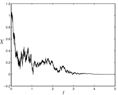
0 1 2 3 4 5 −0.2

0 0.2 0.4 0.6 0.8 1 1.2

t X

Figure 1. The figure shows a stochastic trajectory generated by the Euler–Maruyama scheme for time step4tD10 5_{for the system (5.6).}

Acknowledgments. The authors would like to thank the referee for his or her detailed comments and helpful suggestions.

Bibliography

[1] C. T. H. Baker and E. Buckwar, Numerical analysis of explicit one-step methods for stochastic delay differential equations,LMS J. Comput. Math.3(2000), 315–335. [2] C. T. H. Baker and E. Buckwar, Exponential stability inp-th mean of solutions, and

of convergent Euler-type solutions, of stochastic delay differential equations,J. Com-put. Appl. Math.184(2005), 404–427.

[3] E. Buckwar, Introduction to the numerical analysis of stochastic delay differential equations,J. Comput. Appl. Math.125(2000), 297-307.

[4] E. Buckwar, M. G. Riedler and P. E. Kloeden, The numerical stability of stochastic ordinary differential equations with additive noise, to appear inStoch. Dyn. [5] K. Burrage, P. Burrage and T. Mitsui, Numerical solutions of stochastic differential

equations – implematation and stability issues,J. Comput. Appl. Math.125(2000), 171–182.

[8] D. J. Higham, Mean-square and asymptotic stability of the stochastic theta methods, SIAM J. Numer. Anal.38(2000), 753–769.

[9] D. J. Higham, X. Mao and C. Yuan, Almost sure and Moment exponential stability in the numerical simulation of stochastic differential equations,SIAM J. Numer. Anal. 45(2007), 592–607.

[10] P. E. Kloeden and E. Platen,The Numerical Solution of Stochastic Differential Equa-tions, Springer-Verlag, Berlin, 1992.

[11] R. Sh. Liptser and A. N. Shiryaev,Theory of Martingales, Kluwer Academic Pub-lishers, Dordrecht, 1989.

[12] X. Mao, Approximate solutions for a class of stochastic evolution equations with variable delays—part II,Numer. Funct. Anal. Optim.15(1994), 65–76.

[13] X. Mao,Exponential Stability of Stochastic Differential Equations, Marcel Dekker, New York, 1994.

[14] X. Mao, Stochatic Differential Equations and Applications, Horwood, Chichester, 1997.

[15] X. Mao, LaSalle-type theorems for stochastic differential delay equations,J. Math. Anal. Appl.236(1999), 350–369.

[16] X. Mao, Stochastic versions of the LaSalle theorem,J. Differential Equations153 (1999), 175–195.

[17] X. Mao, The LaSalle-type theorems for stochastic functional differential equations, Nonlinear Stud.7(2000), 307–328.

[18] X. Mao, A note on the LaSalle-type theorems for stochastic differential delay equa-tions,J. Math. Anal. Appl.268(2002), 125–142.

[19] X. Mao, Numerical solutions of stochastic functional differential equations,LMS J. Comput. Math.6(2003) 141–161.

[20] X. Mao, Exponential stability of equidistant Euler–Maruyama approximations of stochastic differential delay equations,J. Comput. Appl. Math.200(2007), 297–316. [21] X. Mao and M. J. Rassias, Khasminskii-type theorems for stochastic differential

de-lay equations,Stoch. Anal. Appl.23(2005), 1045–1069.

[22] X. Mao and C. Yuan,Stochastic Differential Equations with Markovian Switching, Imperial College Press, London, 2006.

[23] S. -E. A. Mohammed,Stochastic Functional Differential Equations, Longman, Har-low, 1986.

[25] A. Rodkina and M. Basin, On delay-dependent stability for vector nonlinear stochas-tic delay-difference equations with Volterra diffusion term,Systems Control Lett.56 (2007), 423–430.

[26] A. Rodkina and H. Schurz, Almost sure asymptotic stability of drift-implicit -me-thods for bilinear ordinary stochastic differential equations inR1_{,J. Comput. Appl.}

Math.180(2005), 13–31.

[27] A. Rodkina, H. Schurz and L. Shaikhet, Almost sure stability of some stochastic dynamical systems with memory,Discrete Contin. Dyn. Syst.21(2008), 571–593. [28] Y. Saito and T. Mitsui, T-stability of numerical scheme for stochastic differential

equations, in:Contributions in Numerical Mathematics, pp. 333–344, World Scien-tific Series in Applicable Analysis 2, World ScienScien-tific, Singapore, 1993.

[29] Y. Saito and T. Mitsui, Stability analysis of numerical schemes for stochastic differ-ential equations,SIAM J. Numer. Anal.33(1996), 2254–2267.

[30] H. Schurz, Preservation of probabilistic laws through Euler methods for Ornstein– Uhlenbeck process,Stoch. Anal. Appl.17(1999), 463–486.

[31] H. Schurz, Almost sure asymptotic stability and convergence of stochastic theta methods applied to systems of linear SDEs inRd_{, to appearRandom Oper. Stoch.}

Equ.

[32] Y. Shen, Q. Luo and X. Mao, The improved LaSalle-type theorems for stochastic functional differential equations,J. Math. Anal. Appl.318(2006), 134–154. [33] A. N. Shiryaev,Probability, Springer-Verlag, Berlin, 1996.

[34] F. Wu and X. Mao, Numerical solutions of neutral stochastic functional differential equations,SIAM J. Numer. Anal.46(2008), 1821–1841.

[35] F. Wu, X. Mao and L. Szpruch, Almost sure exponential stability of numerical solu-tions for stochastic delay differential equasolu-tions,Numer. Math.115(2010), 681–697,

Received October 7, 2010; accepted March 2, 2011. Author information

Fuke Wu, School of Mathematics and Statistics, Huazhong University of Science and Technology, Wuhan, Hubei 430074, P. R. China.

E-mail:[email protected]

Xuerong Mao, Department of Mathematics and Statistics, University of Strathclyde, Glasgow G1 1XH, UK.

E-mail:[email protected]

Peter E. Kloeden, Department of Mathematics, Goethe University, 60054 Frankfurt am Main, Germany.