promoting access to White Rose research papers
White Rose Research Online
Universities of Leeds, Sheffield and York
http://eprints.whiterose.ac.uk/
This is an author produced version of a paper published in Computational Statistics and Data Analysis.
White Rose Research Online URL for this paper: http://eprints.whiterose.ac.uk/3793/
Published paper
Automatic Bandwidth Selection for Circular Density
Estimation
Charles C. Taylor
Dept. of Statistics, University of Leeds, Leeds LS2 9JT, UK
Abstract
Given angular data θ1, . . . , θn ∈ [0,2π) a common objective is to estimate the density. In the case that a kernel estimator is used, band-width selection is crucial to the performance. This paper obtains a “plug-in rule” for the bandwidth, which is based on the concentration of a reference density, namely, the von Mises distribution. It is seen that this is equivalent to the usual Euclidean plug-in rule in the case that the concentration becomes large. In the case that the concentra-tion parameter is unknown, alternative methods are explored which are intended to be robust to departures from the reference density. Simulations indicate that “wrapped estimators” can perform well in this context.
keywords: Angle data; Kernel density estimators; von Mises distri-bution; Ramachandran plot; Smoothing parameter selection.
Contact details: Department of Statistics, University of Leeds, Leeds LS2 9JT, UK,
1 Introduction
Given a random sample of angles θ1, . . . , θn ∈ [0,2π) from some un-known density f(θ) a natural component of exploratory data analysis is to estimate the function f(·). When a parametric form is assumed, this may be achieved by maximum likelihood, or moment-based es-timation. A nonparametric estimator may be naively written as
ˆ
f(θ;h) = 1
n n
X
i=1
Kh(θ−θi) (1)
where Kh(θ) = K(θ/h)/h is a kernel function, usually a symmetric probability density, and h is a smoothing parameter. This kernel esti-mator was first proposed by Fisher (1989) for data lying on the circle, in which he adapted linear data methods of Silverman (1986) and used a quartic kernel function K(θ) = 0.9375(1 − θ2)2. However, when using data on the circle, we cannot use distance in Euclidean space, so all differences θ−θi should be replaced by considering the angle between two vectors:
di(θ) = ||θ−θi|| = min(|θ−θi|,2π − |θ−θi|). (2)
This may also be written as di = cos−1(xTxi) where xT =
(cosθ,sinθ) is a unit vector. A more natural choice for the kernel function is therefore one of the commonly used circular probability densities, such as the wrapped normal distribution, or the von Mises distribution. This leads to an alternative representation for the kernel density estimate (Jammalamadaka and SenGupta, 2001, page 282):
ˆ
f(x;h) = 1
n n
X
i=1
Kh(1−xTxi). (3)
asymp-totic bias and variance of two classes of kernel estimators. This was done by the use of directional derivatives, thus making the results a close analogue of the Taylor series methods used for data in Eu-clidean space.
One of the difficulties in nonparametric density estimation is to make good choices of the smoothing parameter h; see Jones et al. (1996) for an excellent survey of methods. In the Euclidean setting, Silver-man (1986) and Jones et al. (1996) give formulae which depend on derivatives of the unknown density f. When the data lie in Euclidean space, there are many approaches to this problem, a simple exam-ple of which is based on a “Normal-scale rule” or a “rule-of-thumb”. When the kernel function is taken as the gaussian density, this leads to a plug-in selector h = 1.06ˆσn−1/5 (Silverman, 1986). The goal of this paper is to obtain an equivalent plug-in rule for density estimation on the circle.
Specifically, we consider the estimator in which the kernel function is the von Mises density, which gives
ˆ
f(θ;ν) = 1
n(2π)I0(ν)
n
X
i=1
exp{νcos(θ −θi)}. (4)
where Ir(ν) is the modified Bessel function of order r, and the con-centration parameter ν has now taken the role of the (inverse of the) smoothing parameter h. A common approach to obtain the smooth-ing parameter is by considersmooth-ing derivatives of the unknown density and then substituting a “reference” density in order to obtain a plug-in rule; the results of Klemel¨a (2000) could probably be implemented here. However, we instead follow the approach of Marron and Wand (1992) who obtained the form of the exact mean integrated squared error for densities which can be expressed as a mixture of normal densities.
of the concentration parameter of the data (κ), the smoothing param-eter (ν) and the sample size (n). Finally, this can be solved to give a simple plug-in rule for ν dependent only on κ and n. Section 3 dis-cusses robust estimation of κ, suited for the plug-in rule, which may be used in case that the underlying density is not von Mises. Section 4 gives some simulation results, and Section 5 gives a real example using 2-dimensional data from a bioinformatics dataset. We conclude with a discussion.
2 Asymptotic Mean Integrated Squared Error
We suppose f(·) is von Mises (written in general as vM(µ, κ)), with concentration parameter κ and – without loss of generality – mean direction µ = 0. Then the first two moments of (4) are given by
E{fˆ(θ;ν)}= 1
(2π)2I
0(κ)I0(ν)
Z 2π
0 exp{νcos(θ−φ) +κcos(φ)}dφ
= I0{(κ
2 +ν2 + 2νκcos θ)1/2}
(2π)I0(κ)I0(ν)
,
(Jammalamadaka & SenGupta, 2001, p. 40) and
var{fˆ(θ;ν)}= 1
n(2π)2I
0(ν)2
var[exp{ν cos(θ−Θ)}]
= 1
n(2π)2I
0(ν)2I0(κ)
I0{(4ν2+ κ2 + 4κν cosθ)1/2}
−I0{(ν
2+ κ2 + 2κν cos θ)1/2}2
I0(κ)
.
Note that, when ν = 0 we have E{fˆ(θ; 0)}= 1/{(2π)} which does not depend on θ and, in the limit, the estimator is unbiased, i.e.
lim
ν→∞E{fˆ(θ;ν)}= f(θ).
ex-act mean squared error. However, integrating the resulting expression to obtain the exact MISE seems hard to do analytically, so we now derive asymptotic expressions for the above.
As the smoothing parameter ν → ∞ the asymptotic bias is
{2πI0(κ)}−1
exp ν 1 +
κ2
ν2 + 2
κ
ν cos θ
1/2 −1
−exp{κcos θ} +O
ν−2
.
Expanding the square root in a Taylor series, then expanding the exponential function in a Taylor series gives a simpler form of the asymptotic bias as
{4πI0(κ)ν}−1κ2sin2 θexp(κcos θ) +O
ν−2. (5)
Similarly, for large n, and as ν → ∞ the variance has asymptotic form
{4nπ3/2I0(κ)}−1ν1/2exp
2ν
1 +
κ2
4ν2 +
κ
ν cos θ
1/2 −1 +o
ν1/2
n
,
which is valid provided n/ν1/2 → ∞. Again, by expanding the square root, and then the exponential function, as Taylor series, we obtain the simpler form of the asymptotic variance
{4nπ3/2I0(κ)}−1ν1/2exp(κcos θ) +o
ν1/2
n
. (6)
We now integrate the square of the asymptotic bias (5) and the asymp-totic variance (6), to obtain
3κ2I2(2κ)
.
{32πν2I0(κ)2}
and
ν1/2.
2nπ1/2
plug-in rule” for the smoothing parameter ν based on the estimated
κ:
ν = h3nˆκ2I2(2ˆκ){4π1/2I0(ˆκ)2}−1
i2/5
. (7)
Note that this is of a similar asymptotic form as the normal-scale plug in rule when we recall that ν is the concentration parameter, and so takes the role of 1/h2 in h = 1.06ˆσn−1/5. Moreover, if we con-sider the limit as κ → ∞ then the von Mises distribution tends to a Normal distribution, with σ = κ1/2. Hence, in the limit we have
h = ν−1/2 = 1.06κ−1/2n−1/5 which is exactly the same as the usual rule of thumb used for the Normal distribution. A simple method could be to estimate κ from the data, and use equation (7) to select the smoothing parameter for use in (4). Two obvious questions arise at this point: what happens if the data do not come from this reference density (von Mises); how good are all these Taylor series approxima-tions in practice? The next two secapproxima-tions address these quesapproxima-tions in turn.
3 Robust Estimation of Spread
When the data are unimodal, the above selection rule (7) is likely to work reasonably well. However, for bimodal data, the usual estimate of κ – either by maximum likelihood, or the method of moments – may be almost useless. In the most extreme case, an equal mixture of data tightly clustered around φ combined with a similar distribution of data clustered around φ + π will lead to an estimate of κ close to zero. When κˆ = 0 then equation (7) gives ν = 0 which will result in fˆ(θ) ≡ 1/(2π), and so such automatic methods may lead to very misleading density estimates. Indeed, even in the regular case, the maximum likelihood estimator of κ is far from robust, as it has infinite standardized gross error sensitivity (Mardia & Jupp, 1999, p. 276).
Al-ternative robust estimators are also given by Ronchetti (1992) and Ko (1992), but our intention in this paper is to focus on density estima-tion.
In the case of Euclidean data, an alternative rule-of-thumb proposed by Silverman (1986, p. 47) was to take σˆ = min{s,IQR/1.349},
where s is the sample standard deviation, andIQRis the inter-quartile
range. This will work better for bimodal data, and give similar results when the data are normal. This proposal was obtained by compar-ing the population inter-quartile range to the standard deviation. For circular data, if m is the (estimated) median then, for 0 < p < 0.5
define qi(p) ∈ [0, π) such that
p = Z m
m−q1(p)f(θ)dθ =
Z m+q2(p)
m f(θ)dθ
which can be solved for known f(·) and given p. In particular, for the reference (von Mises) distribution, without loss of generality we can set m = 0. The inter p-quantile range for the reference distribution is then given by q2(p) +q1(p) = 2q1(p). The sample circular median is defined (Mardia & Jupp, 1999, p. 17) as the value mˆ such that half the data lies in [ ˆm,mˆ + π) and more data lies closer to mˆ than to
ˆ
m + π. Sample values of qi(p) can then be easily found from the data. The procedure is then as follows:
(1) Select p ∈ (0,1/2)
(2) Form a look-up table which defines q1(p) as a function of κ for the reference distribution vM(0, κ)
(3) Find the sample median mˆ and qˆi(p), i= 1,2 from the data (4) Obtain the estimated κ from the look-up table, using ||mˆ +
ˆ
q2(p)−( ˆm−qˆ1(p))|| where the distance used is as in Equation (2)
An alternative approach is to note that, for the von Mises distribution, the maximum likelihood estimate of κ is obtained from the solution to
A1(κ) =
1
n n
X
i=1
cos(θi−µˆ)
This follows from a more general identity using trigonometric mo-ments which states that Ecos{k(θ − µ)} = Ik(κ)/I0(κ). Thus, al-ternative estimates of κ (for a von Mises distribution) are given by solutions to
Ak(κ) =
1
n n
X
i=1
cos(kθi −µˆk) (8)
where µˆk = tan−1(Psin kθi,Pcos kθi), for k = 1,2, . . .. In the case that the data are von Mises, different values of k will lead to similar estimates of κ. In simulations (not shown), we have observed that κˆk is an increasing function of k, with the bias decreasing, and the variance increasing as κ increases. However, in the case of multi-modal data, then rather different estimates will ensue. Hence, a pos-sible procedure is to estimate κ using k = 1, . . . , K in Equation (8) giving, say, κˆk and then taking κˆ = max{κˆk, k = 1, . . . , K} for use in Equation (7).
4 Simulations
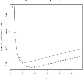
For the standard von Mises distribution, we can compare the average integrated squared error ISE with the approximate MISE given in Section 2, when κ is known. The results, for 500 simulations, and
n = 50 and n = 500 are shown in Figure 1. The approximation looks quite good, improving with n.
We now explore the effectiveness of the plug-in rule, when the data are taken from a mixture of M(≥ 1) von Mises distributions. Specif-ically, we simulate θ1, . . . , θn ∼ f(θ) where the distribution is given by
f(θ) = 1
2π M
X
j=1
pj
exp{κjcos(θ−µj)}
I0(κj)
, i= 1, . . . , n with
M
X
j=1
pj = 1
(9) and we evaluate ISE(ν) = R
( ˆf(θ;ν) − f(θ))2dθ over N = 500
0 2 4 6 8 10
0.01
0.02
0.03
0.04
average and expected integrated squared error
ν
mean integrated squared error
0 5 10 15 20 25
0.005
0.010
0.015
0.020
average and expected integrated squared error
ν
[image:10.595.140.423.92.371.2]mean integrated squared error
ν is obtained for each dataset from the plug-in rule (7) and κˆ is estimated by one of the methods described in Section 3. We also give results when cross-validation is used to select the bandwidth. Here, we select ν to maximize the likelihood cross-validation func-tion LCV(ν) = Q
ifˆ−i(θi;ν), where
ˆ
f−i(θ;ν) =
1
(n−1)(2π)I0(ν) n
X
j6=i
exp{νcos(θ −θj)}
is the leave-one-out estimator. (We have also tried least-squares cross-validation to select the smoothing parameter. The results of this were very similar to, but not quite as good as using likelihood cross-validation, and so are not shown.) Let νCV denote the value of ν
which maximizes LCV(ν). Denote by νK when ν is estimated with
ˆ
κ = max{κˆk, k = 1, . . . , K} and κˆk is the solution to (8). De-note by νp the value of ν when κ is estimated using the inter p -quantile range. We also include results for Fisher’s (1989) adaptation of the quartic kernel, in which his smoothing parameter is given by
hF =
√
7ˆκ−1/2n−1/5, and for a similar method using the Epanech-nikov kernel with hE = 2.345ˆκ−1/2n−1/5. This plug-in rule for a von
Mises density was obtained by using a large concentration approxi-mation for the AMISE solution given by
hE =
120πI0(κ)2
nκ2(2I
0(2κ) +I2(2κ))
1/5
≈ κ−1/2(40√π/n)1/5.
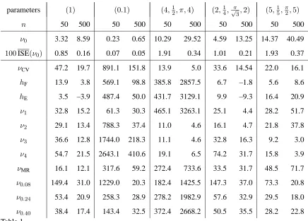
The results are given in Table 1. Note that, for the standard von Mises distribution, if the known κ = 1 is used in (7), then the smoothing parameter is ν = 3.51 for n = 50 and ν = 8.82 for n = 500, whereas if κ = 0.1 then ν = 0.06 for n = 50 and ν = 0.16 for
n = 500, which shows the accuracy of the asymptotic results for finite samples. Note that using the maximum likelihood estimator for
κ with Equation (7) leads to row ν1 in this table.
parameters (1) (0.1) (4,12, π,4) (2,14,√π
3,2) (5, 1 5,
π
2,5)
n 50 500 50 500 50 500 50 500 50 500
ν0 3.32 8.59 0.23 0.65 10.29 29.52 4.59 13.25 14.37 40.49
100ISE(ν0) 0.85 0.16 0.07 0.05 1.91 0.34 1.01 0.21 1.93 0.37
νCV 47.2 19.7 891.1 151.8 13.9 5.0 33.6 14.54 22.0 16.1
hF 13.9 3.8 569.1 98.8 385.8 2857.5 6.7 –1.8 5.6 8.6
hE 3.5 –3.9 487.4 50.0 431.7 3129.1 9.9 –9.3 16.4 20.9
ν1 32.8 15.2 61.3 30.3 465.1 3263.1 25.1 4.4 28.2 51.7
ν2 29.1 13.4 788.3 37.4 11.0 4.6 16.1 4.7 21.8 37.8
ν3 36.6 12.8 1744.0 218.3 11.1 4.6 32.8 16.3 9.2 3.0
ν4 54.7 21.5 2643.1 410.6 19.1 6.5 74.2 31.7 15.8 3.9
νMR 16.1 12.1 317.6 59.2 272.4 733.6 33.5 31.7 48.5 71.7
ν0.08 149.4 31.0 1229.0 20.3 182.4 1425.5 147.3 37.0 73.3 20.8
ν0.24 53.4 20.9 258.3 28.9 278.2 1982.9 57.6 32.9 29.5 18.0
[image:12.595.91.527.70.383.2]ν0.40 38.4 17.4 143.4 32.5 372.4 2668.2 50.5 35.5 28.2 22.8
Table 1
Average integrated squared error results for various bandwidth selection rules. The param-eters of the distribution, given in the top row by (9), are(κ1, p2, µ2, κ2, . . . , pM, µM, κM),
with µ1 = 0in each case. Numerical integration used on 500 grid values; averages taken
over 500 datasets of sizen.ν0 is the smoothing parameter to minimize MISE, and ISE(ν0)
the corresponding minimum. In the lower part of the table we give the percentage increase,
i.e.(ISE(ν•)/ISE(ν0)−1)100% for each method. Here ν• is selected by cross-validation
(νCV), by νK, K = 1,2,3,4 in the case that the wrapped estimator is used, by νp in
the case that the p-quantile range estimator is used, and by νMR in the case that a robust
estimator is used for κ. Two “linear” kernels are also used: hF denotes the performance
for the quartic kernel and respective plug-in rule described by Fisher (1989); hE uses an
Epanechnikov kernel with smoothing parameterhE= 2.345ˆκ−1/2n−1/5.
ν1 (using Equation (7) with κ estimated by Equation (8) with k = 1) gives reasonable answers for both small and moderate κ. The linear kernel estimators are very poorly behaved for large smoothing param-eters (h > π), which occurs when κˆ and/or n are small. An ad hoc solution is simply to rescale the density estimate so that it integrates to unity, but this was not done here. However, note that for moderate
define efficiency for angular kernels.
For the mixtures of distributions, the “standard” plug-in rule ν1 can do very poorly, with both ν2 and ν3 performing similarly, overall, to the cross-validation estimate, but at a cheaper computational cost. In-terestingly, the plug-in bandwidths for the linear kernels can perform surprisingly well for some of the mixtures. Amongst the p-quantile range estimators, ν0.40 performed reasonably, except for one of the mixture distributions.
5 Application to Protein Angles
The backbone of a protein comprises a sequence of atoms
N1−Cα1−C1−N2−Cα2−C2−. . .−Np−Cαp−Cp,
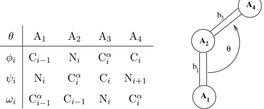
and by choosing 4 atoms with A3 directly behind A2, and A1 directly below A2 (see Table 2) we can specify 3 dihedral angles: φ, ψ, ω.
θ A1 A2 A3 A4
φi Ci−1 Ni Cαi Ci
ψi Ni Cαi Ci Ni+1
ωi Cαi−1 Ci−1 Ni Cαi
A
A
A b
b3
1
2
4
[image:13.595.170.429.412.519.2]1 θ
Table 2
For a sequence of atoms (A1, A2, A3, A4) as specified, with A3 directly behind A2, and
A1 directly below A2 , we label the angle shown in the sketch as one of φ, ψ, ω.
The angle ω is restricted to be about zero, and is of little interest. The remaining angles (φ, ψ) are measured between −π and π. A scatter plot of a collection of(φi, ψi), i = 1, . . . , nfor a protein is known as a
Ramachandran plot, and has been used to characterize the secondary
structure of the protein.
independent components, and common concentration κ, then we can approximate the asymptotic integrated variance of the kernel density estimate as ν/(4nπ) with asymptotic integrated bias-squared as
κ2h
3I0(2κ)I2(2κ) +I1(2κ)2
i .
(32π2I0(κ)4ν2) .
Hence in this case, the rule of thumb is
ν = h
nκˆ2n
3I0(2ˆκ)I2(2ˆκ) +I1(2ˆκ)2
o .
(4πI0(ˆκ)4)
i(1/3)
. (10)
We illustrate a kernel density estimate for the protein Malate
dehy-drogenase which has n = 343 observations; the Ramachandran plot is shown in Figure 2. For the purposes of this example, we assume that the sequence of angles are independent. To obtain ˆκ we use the geometric mean of the estimated concentrations of the marginal data (using the wrapped estimate with K = 3). We obtain ˆκ = 5.69 and so, using Equation (10), we use smoothing parameter ν = 36.85 in a multiplicative kernel. A contour plot of the square root — the trans-formation was used in order to reveal more of the detail — of the estimated density is shown in Figure 2.
−3 −2 −1 0 1 2 3
−3
−2
−1
0
1
2
3
Malate dehydrogenase
φ
ψ
contours of sqrt(density estimate)
φ
ψ
−3 −2 −1 0 1 2 3
−3
−2
−1
0
1
2
[image:14.595.95.486.484.666.2]3
6 Concluding Remarks
Extending some of the above results to a mixture of von Mises dis-tributions would also be straightforward, and would proceed along the lines of Marron & Wand (1992). However, although we could ob-tain expressions for the approximate MISE, it would depend on the mixing proportions (as well as the means and concentrations of each component), and no plug-in rule would be readily available.
Agostinelli (2007) has considered alternative approaches to the robust estimation of κ which could also be used in Equation (7) in place of those considered here.
Finally, we note the survey paper of Jones et al., (1996) which dresses the issue of bandwidth selection for real-valued data. In ad-dition to the ideas of the current paper, there are several alternatives which will have a counterpart for directional data. In particular, there are now well-known results in the euclidean case which obtain more sophisticated plug-in rules by estimating functionals of the deriva-tives. By using the results of Klemel¨a (2000) it should be possible to obtain circular data counterparts.
Acknowledgements
I would like to thank John Kent and Kanti Mardia for useful discus-sions.
References
Agostinelli, C. (2007). Robust Estimation for circular data.
Compu-tational Statistics and Data Analysis, (in press).
Fisher, N.I. (1989). Smoothing a sample of circular data. Journal of
Hall, P., Watson, G.S. and Cabrera, J. (1987). Kernel density estima-tion with spherical data. Biometrika, 74, 751–762.
Jammalamadaka, S. Rao and SenGupta, A. (2001). Topics in Circular
Statistics. World Scientific, Singapore.
Jones, M. C., Marron, J.S. and Sheather, S. J. (1996). A Brief survey of Bandwidth selection for density estimation. Journal of the
Ameri-can Statistical Association, 91, 401–407.
Klemel¨a, J. (2000). Estimation of densities and derivatives of densi-ties with directional data. Journal of Multivariate Analysis, 73, 18– 40.
Ko, D. (1992). Robust estimation of the concentration parameter of the von-Mises distribution. The Annals of Statistics, 20, 917–928.
Mardia, K.V. and Jupp, P. E. (1999). Directional Statistics. John Wi-ley, Chichester.
Marron, J. S. and Wand, M. P. (1992). Exact mean integrated squared error. The Annals of Statistics, 20, 712–736.
Ronchetti, E. (1992). Optimal robust estimators for the concentration parameter of a von Mises-Fisher distribution. In The Art of Statistical
Science. A tribute to G.S. Watson, ed: K.V. Mardia, pp. 65–74.
Silverman, B. W. (1986). Density Estimation for Statistics and Data