Model-Based Networked Control System Stability
Based on Packet Drop Distributions
Lanzhi Teng, Peng Wen, and Wei Xiang Faculty of Engineering and Surveying
University of Southern Queensland West Street, Toowoomba, QLD 4350, Australia
{teng,wen,xiangwei}@usq.edu.au
Abstract—This paper studies the system stability of a Model-Based Networked Control System in the cases where packet losses follow a certain distributions. In this study, the unreliable nature of network links is modelled as a stochastic process. This process provides us two system structures, representing packets dropped and received respectively. This new system with two structures is asymptotically stable, if the plant model is updated with the data from plant within the maximum interval and the packet drop follows discrete distributions with finite expectations such as Uniform Distribution and Bernoulli distribution. If the packet loss follows discrete distributions with infinite expectation such as Poissonian Distribution, the stochastic system is stable when the biggest interval is limited to the maximal update time interval. These results are verified in simulations.
Keywords—Packet Drop Distribution, Model-Based Networked Control System, System Stability
I.INTRODUCTION
Networked control systems (NCSs) have attracted considerable amount of attention in the past decade. Compared with traditional feedback control systems, NCSs reduce the system wiring, make the system easy to operate, maintain and diagnose in case of malfunctioning. In spite of the great advantages that the networked control architecture brings, inserting a network between the plant and the controller introduces many problems as well. Network induced delays are unavoidable because of the scheduling schemes. Packet drops occur sometimes because of network congestions. Unlimited data rate is not possible because of finite bandwidth available. In [1-2], system stability has been studied while network time delays are considered. Vijay Gupta, Babak Hassibi and Richard M. Murry in [3], investigated the system performance with packet drops, and concluded that packet drops degrade a system’s performance and possibly cause system instability. In [4], John K. Yook, Dawn M. Tilbury and Nandit R. Soparkar used state estimator techniques to reduce the communication volume in a networked control system.
Packet drop over a network exhibits stochastic behavior. The network can be described as there is some correlation between consecutive packets in term of Markov Chain. In [5-6] H∞ filtering for a class of uncertain Markovian jump linear systems is investigated. A Markovian jumper linear filter is given in terms of linear matrix inequalities. Optimal Kalman filters are used in Markov jump linear systems as the estimator, and the linear matrix inequality in the bounded real lemma is given as both necessary and sufficient in [7-8].
In NCS, we consider the communication between the sensor and the controller or estimator is subject to unpredictable packet loss. We assume that if a packet dropped, a new observation is taken. In [9], Montestruque proposed a Model-based NCS, and provided the necessary and sufficient conditions for stability in terms of the update time and the parameters of the plant and its model, assuming that the frequency at which the network updates the state in the controller is constant.
In the authors’ best knowledge, the packet drop distribution has not been fully investigated. This work studies system stability in the cases where packet drops follow different distributions. We model the unreliable nature of the network links as a stochastic process, and assume that this stochastic process is independent of the system initial condition and the plant model state is updated with the plant state at the time when packet arrives. Then, a model for the model-based NCS is built up and a new system matrix is obtained regarding the intervals between the arrived packets following random distributions. The result of our study shows that the system is stable as long as the system error is reset within the maximum update time. Our further study also shows that the distributions of the packet drops affect the system stability. This conclusion is demonstrated in examples at the end.
This paper is organized as follows. In section 2, system model is set up in the form of packet losses. In section 3, system stability is analyzed in the cases where packet drops follow different distributions. In section 4, example is provided to verify our conclusion. Conclusion is drawn in section 5.
II.SYSTEM DESCRIPTION
A model-based control system in Fig. 1 is considered, where the plant is given as:
)
(
)
(
)
1
(
n
Ax
n
Bu
n
x
+
=
+
(1)where x(n) is the plant state vector. A, B are system parameter matrices.
A model of the plant is built up to provide the estimated plant state vector. The plant model dynamics is given by:
)
(
ˆ
)
(
ˆ
ˆ
)
1
(
ˆ
n
A
x
n
B
u
n
x
+
=
+
(2)A
A
A
~
=
−
ˆ
, andB
~
=
B
−
B
ˆ
, representing the difference between the plant and the model.We consider only state feedback controller, which is given by:
)
(
ˆ
)
(
n
L
x
n
u
=
(3)where L is the controller feedback gain matrix. We assume that the dynamic model is subject to the same control signal u(n) as the original system.
III.STABILITY ANALYSIS
As the packets are sent through a network from the plant to the controller, the packet drops happen randomly. Periods of packet streams are interrupted by periods without packets received. The intervals between the received packets vary with a distribution. The lengths of interval depend on the QoS of the network.
The stochastic process
{ }
γ
n models the unreliable nature of the network links. We assume thatγ
n is independent of the initial condition, x(0). We reuse the previous packet if a packet is not received. The vectorx
(
n
)
is current state x(n) with probability p if a packet is received. That gives us the following equation:)
(
)
(
n
x
n
x
=
γ
n (4) Although the control packets may not be received by the plant, we make the assumption that the model will always know without delay whether or not the control packet was received. We define the state error as:)
(
ˆ
)
(
)
(
n
x
n
x
n
e
=
−
(5)We assume that the plant model state
x
ˆ
(
n
)
be updatedwith the plant’s state
x
(
n
)
atevery
n
k, wheren
k−
n
k−1=
h
k,h
k is the interval betweenthe received packets, k=0, 1, 2, ... Then,
e
(
n
k)
=
0
.Now we can write the evolution of the closed loop NCS,
=
+
+
)
(
)
(
)
(
)
1
(
)
1
(
n
e
n
x
A
n
e
n
x
nγ
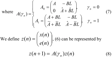
(6)where = − + − + = = + − = = 1 , ~ ˆ ~ ~ 0 , ˆ ˆ 0 ) ( 1 0 n n n L B A L B A BL BL A A L B A BL A A A γ γ
γ (7)
We define
=
)
(
)
(
)
(
n
e
n
x
n
z
, (6) can be represented by)
(
)
(
)
1
(
n
A
z
n
z
+
=
γ
n (8) We modeled the system as a set of linear systems, in which the system jumps from one mode representing byA
0 toanother representing by
A
1. We define matrixΛ
as the function ofA
0,A
1, p andα
)
,
,
,
(
A
0A
1p
α
f
=
Λ
(9)where p is the probability of the interval between the received packets,
α
is the packet drop rate.On the interval,
n
∈
[
n
k,
n
k+1)
, the system described by (8) has the following response) ( 0 ) ( ) ( ) ( )
( n n k nn k
n z n x n e n x n
z −k =Λ−k
Λ = =
Note that at time
n
k,
=
0
)
(
)
(
k kn
x
n
z
, that is the error)
(
n
ke
is reset to zero. We can represent this by)
(
0
0
0
)
(
−
=
kk
z
n
I
n
z
, here I is the unit matrix with properdimensions and
z
(
n
k−)
=
Λ
hkz
(
n
k−1)
, we have)
(
0
0
0
)
(
Λ
−1
=
h kk
z
n
I
n
z
k .If at
n
=
n
0 the initial condition
=
0
)
0
(
)
0
(
x
z
, thesystem response is:
[image:2.595.320.554.90.211.2])
0
(
0
0
0
0
0
0
...
0
0
0
0
0
0
...
)
(
0
0
0
0
0
0
)
(
0
0
0
)
(
1 1 2 1z
I
I
I
I
n
z
I
I
n
z
I
n
z
h h n n k h h n n k h n n k k k k k k k
Λ
Λ
Λ
=
Λ
Λ
Λ
=
Λ
Λ
=
− − − − − − L x(n)Figure 1 Model-based Networked Control System Model Model
Plant
u(n) x(n)
x(n) ^
-
u(n)i.e.
) 0 ( 0 0
0 0
0 0 ... 0 0
0 0
0 0 )
(n I I I 1 I z
z n nk hk h
Λ Λ Λ
= − (10)
The update time
h
k vary randomly. The frequency at which the network updates the state is not constant. The packet loss may obey different distributed statistical processes. The distribution of intervals, representing byh
k , may follow Bernoulli Distribution process, Uniform Distribution, Poissonian Distribution, etc. We categorize the case update timeh
k>
h
0 as time delay, andh
k>
h
max as packet loss,where
h
0 is data interval without packet loss,h
max is themaximal update time.
h
k>
h
max will cause the system instable.A. Bernoulli Distribution
Basically, random variable,
γ
n=
0
, when this link fails, i.e. the packet is lost,γ
n=
1
, otherwise.γ
n takes value 0 with small probabilityα
, representing packets dropped to yield a interval between the received packets, andγ
n takes value 1 with big probability1
−
α
, representing no packet dropout.α
is a known constant. Fig. 2 shows the probability function of a Bernoulli distribution.The probability mass function of this distribution is
1
0
,
1
,
)
Pr(
1 0
=
=
−
=
=
=
k
k
k
p
i n iα
α
[image:3.595.314.544.232.324.2]γ
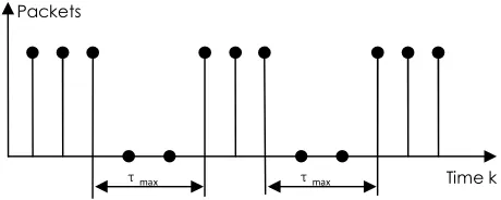
(11)Fig. 3 shows that a stream of packets is interrupted with a interval of certain length without packets.
We define
Λ
=
α
A
0+
(
1
−
α
)
A
1 to model the jump system in case the packet loss obeys Bernoulli Distribution process. In (10), if the interval between the received packetsk
h
is less than the maximum update time,h
max, there are packets arrived from the plant to update the model states before the system become instable. Then, the system keeps stable. Whenh
k>
h
max, packet loss, the system becomes instable.B. Uniform Distribution
The adjacent packets may be received in a period, following consecutive packets drop out as shown in Fig. 4.
The length of intervals between the received packets may vary. We assume that the interval variable X has any of n possible values,
k
1,k
2, …,k
n that are equally possible. Theprobability of any outcome
k
i, is 1/n, where i=1, 2, …, n. The probability function is defined only at integer values of i as following.n
k
X
p
i i1
)
Pr(
=
=
=
(12)Fig. 5 is the probability mass function in Uniform Distribution. The connecting lines are only guides for the eye and do not indicate continuity.
We define
1 0
0
0
)
(
1
)
1
...
1
1
(
A
A
n
A
n
A
n
n
α
α
+
+
+
+
−
=
Λ
4
4
4
4
3
4
4
4
4
2
1
to model the jump system in case the packet loss obeys
Uniform Distribution process. We have
1
0
(
1
)
A
A
α
α
+
−
=
Λ
, whereα
is the data dropout rate. In ProbabilityK0 K1
γ
n1-α
Figure 2 Probability Mass Function in Bernoulli Distribution
α
Time k
hk
[image:3.595.318.441.509.596.2]Packets
Figure 3 A Packet Stream in Bernoulli Distribution
Time k
Figure 4 A Packet Stream in Uniform Distribution
τmax
Packets
τmax
Probability
K1 K2 kn X
1/n
[image:3.595.51.285.599.689.2]
[image:3.595.320.514.631.681.2](10), if the interval between the received packets is less than the maximum update time,
h
max, there are packets arrived from the plant to update the model states. The system is stable. To keep the system stable,τ
max<
h
max, whereτ
max is the biggest interval.C. Poissonian Distribution
If packet loss obeys a Poisson distributed statistical process, i.e. if successive packet loss is independent and obeys normal counting statistics, in a sequence of n packets the interval variable X has any of n possible values,
k
1,k
2 , …,k
nprobabilities
p
i, where i=1, 2, …, n. The probability function is defined only at integer values of i as following!
)
Pr(
i k
i i
k
e
k
X
p
i λ
λ
−=
=
=
(13)where e is the base of the natural logarithm (e = 2.71828...),
!
i
k
is the factorial ofk
i, λ is the average value of X.Fig. 6 is the probability mass function in Poissonian Distribution.
We define 0 1
1 0
1
)
1
(
)
(
p
A
p
A
A
n
k i
i k
i i
m m
α
α
+
+
−
=
Λ
∑
∑
+ = =
to model the jump system in case the packet loss obeys Poissonian Distribution process. Then, we have
1
0
(
1
)
A
A
α
α
+
−
=
Λ
, whereα
is the data dropout rate. In (10), if the interval between the received packets is less than the maximum update time,h
max, the system is stable. To keepthe system stable,
τ
max<
h
max, whereτ
max is the biggest interval. However, the interval variable is attributed to a discrete distribution with infinite as shown in Fig. 7, packets drop out at random points in time. At some points the adjacent packets may be received without interval between the packets. At some points packets may be dropped with bigger or smaller interval between the received packets. Whenn
→
∞
, the interval may be infinite with a very small probability. i.e.∞
→
max
τ
. We may find a margin value among the intervals between the received packets,τ
m≈
h
max , whenX
=
k
m. When the interval is less than this margin value,τ
m , thesystem stays stable. When the interval is greater than the maximum update time,
τ
max, the system becomes instable.From the distributions we can see that if the random variable X, which represents the intervals between the packets, is attributed to a discrete distribution with finite expectation such as Uniform Distribution and Bernoulli Distribution, the system keeps stable when the biggest interval is less than the update time,
τ
max<
h
max. If X is attributed to a discrete distribution with infinite expectation such as Poissonian Distribution, the system keeps stable for the periodsτ
<
τ
m and becomes instable for the periodsτ
>
τ
m.IV.SIMULATIONS
In order to experimentally verify the correctness of the above analysis, we used a simple feedback control system to estimate the system response in case of packet loss. We now present an example of a full state feedback as following:
)
(
1
0
)
(
1
0
1
1
)
1
(
n
x
n
u
n
x
+
=
+
with the state feedback law
(
1
2
)
ˆ
(
)
)
(
n
x
n
u
=
−
−
We design a plant model using a random perturbation of the original plant matrices:
)
(
8578
.
0
4189
.
0
)
(
ˆ
0056
.
1
2410
.
0
6636
.
1
3626
.
1
)
1
(
ˆ
n
x
n
u
n
x
+
−
=
+
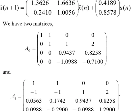
We have two matrices,
− −
=
7100 . 0 0988 . 1 0 0
8258 . 0 9437 . 0 0 0
2 1
1 0
0 0
1 1
0
A
and
− −
− −
=
2900 . 1 0988 . 0 2900 . 0 0988 . 0
8258 . 0 9437 . 0 1742 . 0 0563 . 0
2 1
1 1
0 0
1 1
1
A .
Probability
[image:4.595.314.540.125.212.2]K1 K2 … λ … kn X
Figure 6 Probability Mass Function in Poisson Distribution
Km
[image:4.595.53.284.362.465.2]Time k Packets
Figure 7 A Packet Stream in Poissonian Distribution
[image:4.595.316.544.538.731.2]We assume there is no packet dropout and the frequency at which the network updates the state is constant. Fig. 8 is a plot of magnitude of the maximum eigenvalues of
Λ
0
0
0
0
0
0
I
I
hagainst update time h. From the graph it
can be seen that the maximum value for h is
h
max=
4
. For4
>
h
, the NCS has eigenvalues with magnitude larger than one and therefore will be unstable.0 1 2 3 4 5 6 7 8 9 10
0 0.5 1 1.5 2 2.5 3 3.5 4 4.5
Update Time h
M
a
x
e
ig
e
n
v
a
lu
e
In the simulation, the system jumps from one mode with h>4, representing by
A
0 to another mode with h≤4,representing by
A
1. Table 1 shows the algorithm.Given plant matrices, model matrices, and corresponding discrete distribution
1. Form the matrices
A
0 andA
1 according to the control scheme2. Produce the random numbers, simulating the packet intervals, according to the different discrete distribution
3. Apply different matrices to calculate the system response according to different packet intervals
if h>4
0 0
0 0
0 0
0 I A
I h
else
0 0
0 0
0 0
1 I A
I h
end
4. Plot the system response
Fig. 9-11 show the plots of the system responses with initial
condition
=
0
0
1
1
)
0
(
z
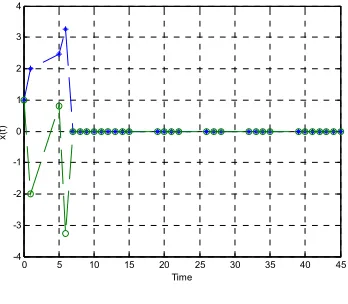
in case the packet intervals areattributed to Bernoulli Distribution, Uniform Distribution, and Poissonian Distribution, respectively.
The random numbers, simulating Bernoulli Distribution packet intervals, are as follows, 1, 4, 1, 1, 1, 1, 1, 1, 1, 1, 1, 1, 4, 1, 1, 1, 4, 1, 1, 4, 1, 1, 1, 4, 1, 1, 1, 1, 1.
0 5 10 15 20 25 30 35 40 45
-4 -3 -2 -1 0 1 2 3 4
x
(t
)
Time
The random numbers, simulating Uniform Distribution packet intervals, are as follows, 2, 3, 3, 2, 2, 4, 3, 3, 4, 3, 4, 1, 1, 3, 3, 2, 2, 1, 4, 1, 3, 1, 1, 3, 4, 3, 4, 3, 3, 2.
0 10 20 30 40 50 60 70 80
-0.2 0 0.2 0.4 0.6 0.8 1 1.2
x
(t
)
Time
The random numbers, simulating Poisson Distribution packet intervals, are as follows, (a) 1, 3, 2, 3, 1, 1, 3, 3, 2, 1, 1, 2, 1, 4, 2, 2, 2, 2, 1, 2, 1, 1, 2, 2, 2, 3, 2, 2, 2, 3; (b) 8, 8, 3, 3, 4, 4, 3, 3, 4, 4, 4, 5, 5, 5, 6, 4, 7, 5, 1, 4, 5, 2, 8, 8, 4, 5, 4, 6, 7, 2.
Figure 10 The System Response with Uniform Distribution Packet Intervals
Figure 9 The System Response with Bernoulli Distribution Packet Intervals
[image:5.595.52.196.209.320.2]Figure 8 The Plot of Magnitude of the Maximum eigenvalues of the Test Matrix
[image:5.595.321.495.241.393.2] [image:5.595.60.274.455.717.2] [image:5.595.321.497.468.620.2]0 5 10 15 20 25 30 -2
-1.5 -1 -0.5 0 0.5 1 1.5 2
x
(t
)
Time
0 20 40 60 80 100 120
-0.5 0 0.5 1 1.5 2 2.5x 10
4
x
(t
)
Time
From the above simulation results we can see that if the packet intervals are attributed to a discrete distribution with finite support such as Uniform Distribution and Bernoulli Distribution, the system keeps stable when the biggest interval is less than the update time. If they are attributed to a discrete distribution with infinite support such as Poissonian Distribution, the system keeps stable in finite time. When time increases, the packet interval range increases. Then, the system becomes instable.
V.CONCLUSION
In this paper, the stability problem in NCS with unpredictable packet drops has been investigated. The result of our study shows that the system is stable as long as the system error is reset within the maximum update time. Our further study also shows that the distributions of the packet drops affect the system stability. If the packet drop follows discrete distribution with finite expectations such as Uniform Distribution and Bernoulli distribution, the system is asymptotically stable when the maximum time interval between the received packets is under the maximum update time. If the packet loss follows discrete distribution with infinite expectation such as Poisson Distribution, the stable stochastic system is asymptotically stable, when the maximum time interval between the received packets is limited to the maximal update time. This conclusion is demonstrated in examples at the end.
REFERENCES
[1] Minrui Fei, Jun Yi, and Huosheng Hu, “Robust Stability Analysis of an Uncertain Nonlinear Networked Control System Category”, International Journal of Control, Automation, and Systems, Vol. 4, No. 2, pp. 172-177, Apr. 2006.
[2] Johan Nilsson, “Real-Time Control Systems with Delays”, PhD Thesis, University of Toronto, Canada, 2003.
[3] Vijay Gupta, Babak Hassibi and Richard M. Murry, “Optimal LQG Control across Packet dropping Links”, System & Control Letters, June 2007, Vol 56, pp. 439-446.
[4] John K. Yook, Dawn M. Tilbury and Nandit R. Soparkar, “Trading Computation for Bandwidth: Reducing Communication in Distributed Control Systems Using State Estimators”, IEEE Transactions on Control Systems Technology, July 2002, Vol 10, No. 4, pp. 503-518.
[5] Carlos E. de Souza and Marcelo D. Fragoso, “Robust H∞ filtering for uncertain Markovian jump linear systems”, International Journal of Robust and Nonlinear Control, Vol. 12, pp. 435 – 446, Jan 2002. [6] Marcelo D. Fragoso and Carlos E. de Souza, “H∞ filtering for
Markovian jump linear systems”, The 35th conference on Decision and Control, Kobe, Japan, December 1996.
[7] A. K. Fletcher, S. Rangan, and V. K Goyal, “Estimation from Lossy Sensor Data: Jump Linear Modelling and Kalman Filtering”, Third International Symposium on Information Processing in Sensor Networks, Berkeley, California, USA, 26-27 Apr. 2004, pp. 251-258. [8] Alyson K. Fletcher, Sundeep Rangan, Vivek K Goyal, and Kannan
Ramchandran, “Robust Predictive Quantization: A New Analysis and Optimization Framework”, ISIT 2004, Chicago, USA, June 27-July 2, 2004, pp. 429.
[9] Luis A. Montestruque, “Model-Based Networked Control Systems”, PhD Thesis, University of Notre Dame, November 2004. Figure 11 The System Response with Poissonian
Distribution Packet Intervals
[image:6.595.58.236.96.237.2]