R E S E A R C H
Open Access
Networked iterative learning control for
discrete-time systems with stochastic packet
dropouts in input and output channels
Jian Liu and Xiaoe Ruan
**Correspondence:
[email protected] Department of Applied Mathematics, School of Mathematics and Statistics, Xi’an Jiaotong University, Xi’an, P.R. China
Abstract
The paper develops a derivative-type (D-type) networked iterative learning control (NILC) scheme for repetitive discrete-time systems with packet dropouts
stochastically occurred in input and output communication channels. The scheme generates the sequential recursive-mode control inputs by mending the dropped instant-wise output with the synchronous desired output, while it drives the plant by refreshing the dropped instant-wise control input with the used consensus-instant control input at the previous iteration. By adopting statistic technique, the
convergences of the developed NILC scheme for linear and nonlinear systems are derived, respectively. The derivations present that under certain conditions the mathematical expectations of the stochastic tracking errors in the sense of 1-norm converge to zero. Numerical simulations exhibit the effectiveness and validity.
Keywords: iterative learning control; mathematical expectation; networked control systems; stochastic packet dropouts
1 Introduction
In biology, psychology, sociology as well as in philosophy, the notion of ‘learning’ has been acknowledged as one of intelligent capabilities for an individual to earn food and fit the environment for surviving and evolving persistently. It is noted as a process for an in-telligent agent to acquire knowledge or experience from its perception and cognition of the environment and then to act on the environment so as to improve its behavior per-formance at the next time. Benefited from the advancing computer technology, learning algorithm has been algorithmically embedded into the control programming of a robotic manipulator to track a desired trajectory. The pioneer contribution is the iterative learn-ing control (ILC) invented in the s whose scheme is to utilize the historical tracklearn-ing discrepancy to modify its control command so that the upgraded control command may drive the repetitive system to track a predetermined desired trajectory []. Overviewing the existing ILC investigations, the ILC has been acknowledged as one of the most effec-tive intelligent control strategies for a repetieffec-tive system operated over a fixed time interval owing to its less system information requirement and precise tracking insurance [–].
Along with the development of internet service, some of efficacious control schemes can be networked for higher efficiency and lower cost, which forms networked control
systems (NCSs). However, confined by the physical features of the wire or wireless net communication devices such as the limit bandwidth or temporal oscillation of the net, the embedment of the communication net into the traditional control loop may possi-bly incur the communication delay and packet dropout which will deteriorate the control effects [–]. In terms of the communication delays, a usual manner is to replace the delayed data by the captured data at the last sampling instant in the case when the delay is within one sampling step length [–]. In treating the packet dropout, the method is to replace the dropped data with the latest captured one [, ]. It has been shown that the aforementioned handling methods work satisfactorily under the assumptions that the probabilities of the communication delay and the packet dropout are constrained appro-priately.
Inspired by the handling methods for the NCSs, the investigations have been emerged to embed the network into the conventional ILC system addressing the communication delay and/or packet dropout. In detail, a D-type NILC strategy has been considered for a class of linear time-invariant (LTI) multiple-input-multiple-output (MIMO) systems, where both the packet dropout and the communication delay of the system output are considered []. Reference [] has addressed a proportional-type (P-type) NILC for a class of nonlinear systems with random packet losses happening in both the input and the output communication channels, where the term ‘packet losses’ is no other than commu-nication delays. The handling methods for the delayed data in [, ] are to substitute the one-step-delayed data by the captured data at the last sampling instant, which is no other than the conventional NCSs [–]. As the above-mentioned replacement mecha-nism of the communication delayed data is one-step-ahead mode, it to some extent does not match the ILC scheme which is an exact time point-to-point mapping along iteration direction. As shown in [, ], the tracking error is asymptotically upper-bounded but nonzero when communication delays occur. In addition, one [] has developed a P-type NILC scheme for a class of nonlinear systems with stochastic delays happened in both sys-tem output and control input communication channels, where the delayed data is replaced with the synchronous data of the previous iteration. It has been shown that the proposed NILC scheme can drive the NILC system to track the desired trajectory precisely as the iteration goes on.
the iteration axis. Under the assumption that for a fixed sampling instant the quantity of the successive packet loss is less than a constant, the learning gain has been designed as an iteration-decreasing sequence and the convergence has been deduced by stochas-tic approximation and optimization techniques. In further work [] one has considered the NILC design for nonlinear systems with unknown control direction and system out-put packet dropouts. It is recalled that the handling strategy of dropped data proposed in [–] is equivalent to replacing the dropped data with the synchronous desired output signal. Meanwhile, [] has developed an NILC scheme by replacing the dropped output with the successfully captured latest synchronous output.
It is observed that, however, the literature [–] only considers the packet dropout curring in the output communication channel. As a matter of fact, the packet dropout oc-curs not only in the output communication channel, but also possibly in the input commu-nication channel. Under this circumstance, the synchronous desired signal replacement in the existing literature [–] is hardly adoptable for the input dropout as the desired input is unavailable but pursued. Nevertheless, it is worth recalling that the learning ca-pability of the ILC is principally benefited from the time point-to-point compensation for the control input along the iteration direction rather than the time axis. Thus, the replace-ment for the dropped data by the captured latest synchronous ones would be a feasibility to deal with the dropped input. This motivates the paper.
This paper is to develop a D-type NILC strategy for discrete-time systems with both stochastic input and output packet dropouts. The strategy mends the dropped wise output with the synchronous desired output, while it refreshes the dropped instant-wise input with the consensus-instant input used at the previous iteration. By means of the statistic technique, the convergence of the developed NILC scheme for respective linear and nonlinear systems is derived, which shows that under certain conditions the mathe-matical expectations of the stochastic tracking errors in the sense of -norm converge to zero.
The rest of the paper is organized as follows. In Section , a P-type NILC scheme is formulated and some notations are presented. Section analyzes the convergence of the proposed NILC scheme to linear systems and Section addresses the convergent char-acteristic of the proposed NILC scheme imposed on a kind of affine nonlinear systems. The effectiveness and the validity are numerically simulated in Section and Section concludes the paper.
2 NILC algorithm and notations
Let (X,F,P) be a probability space andp∈[, ] be a constant number, whereX={, } is a sample space, F ={∅,{},{},{, }}is a set of events and P is a probability mea-sure on setF satisfyingP(∅) = ,P({}) =p,P({}) = –pandP({, }) = , respectively. A stochastic variableξ is said to be subject to - Bernoulli distribution refers thatξ is defined on (,F,P) satisfyingξ() = andξ() = . DenoteE{ξ}as the mathematical ex-pectation of the stochastic variableξ. Then E{ξ}=P(ξ= ) = –p. Letx= (x, . . . ,xn)
andy= (y, . . . ,yn)∈Rnbe two n-dimensional real vectors. The partial order relation
≺is defined as x≺yif and only ifxi≤yifor alli= , , . . . ,n. LetH= (hij)m×n∈Rm×n
be a real matrix. Denote |x|= (|x|,|x|, . . . ,|xn|), |H|= (|hij|)m×n, x=ni=|xi|and
H=max≤j≤n
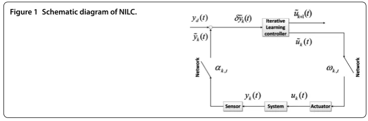
Figure 1 Schematic diagram of NILC.
Consider a class of repetitive discrete-time single-input-single-output (SISO) systems described as follows:
xk(t+ ) =f(xk(t),uk(t)), t∈S–,
yk(t) =g(xk(t),uk(t)), t∈S,
()
where the subscriptk= , , . . . denotes the iteration index,trefers to the discrete-time variable withS–={, , , . . . ,N– }andS={, , , . . . ,N}.x
k(t)∈Rn,uk(t)∈Randyk(t)∈
Raren-dimensional state, scalar input and scalar output at thekth iteration, respectively. f(·,·) andg(·,·) are functions of the state and input variables.
In the system (), when the control inputuk(t) is generated by an ILC update law and
is transmitted from the ILC unit to the actuator via the input communication channel for driving the system, and simultaneously the system outputyk(t) is transferred through
the output communication channel from the sensor to the ILC unit for data updating, the mode is regarded as a networked iterative learning control paradigm, abbreviated as NILC. The diagram of the NILC is illustrated in Figure . In the schematic diagram,u˜k(t)
denotes the signal which is transmitted from the ILC unit to the actuator via the input net channel. Its stochastic dropout is regarded as a random on/off switch.uk(t) refers to
the control command of the actuator for driving the system which is composed ofu˜k(t)
anduk–(t) in a switch mode. In detail, in the case when the ILC signalu˜k(t) attinstant is
successfully captured by the actuator, the signalu˜k(t) is directly taken asuk(t) for driving
the system, while in the case when the ILC signalu˜k(t) attinstant is dropped, the actuator
will borrow its used input datauk–(t) at the previous iteration for driving the system.
Mathematically, the control inputuk(t) of the actuator is represented as follows:
u(t) =u˜(t), t∈S–, given as a test signal,
uk(t) =ωk,tu˜k(t) + [ –ωk,t]uk–(t), t∈S–,k= , , . . . ,
()
where for allt∈S– andk= , , . . . ,ω
k,t is a stochastic variable subject to - Bernoulli
distribution. Here,ωk,t = means that the signalu˜k(t) is successfully transmitted while
ωk,t= marks that the signalu˜k(t) is dropped.
Analogously,yk(t) refers to the system output which will be transmitted to the ILC unit
for data updating through the output channel and its stochastic dropout is considered as a random off/on switch. Whilsty˜k(t) is a candidate signal for the ILC updating which will
be either the system outputyk(t) or the desired signalyd(t) depending on the success of
the data communication, namely, in the case when the system outputyk(t) is successfully
the system outputyk(t) is dropped, the ILC unit will utilize the saved desired output signal
for the new command generation. Thus, the signal˜yk(t) is formulated as follows:
˜
yk(t) =αk,tyk(t) + [ –αk,t]yd(t), t∈S+,k= , , . . . , ()
whereS+={, , . . . ,N},y
d(t) is the desired output, and for allt∈S+andk= , , . . . ,αk,tis
a stochastic variable subject to - Bernoulli distribution.
Remark As shown in () and (), the handling methods of packet dropouts is differ-ent from those in [, ]. The handling methods of packet dropouts in [, ] can be described as follows:
uk(t) =ωk,tu˜k(t) + [ –ωk,t]uk(t– ),
˜
yk(t) =αk,tyk(t) + [ –αk,t]y˜k(t– ).
Meanwhile, the replacement algorithm () is also different from (). This benefits from the characteristic of ILC and it is expected that the replacement algorithms () and () show better performance.
It is noted that in the concerned NILC profile Figure , the status of the communicated data packet is either dropped or captured in success, which is modeled as a - Bernoulli stochastic variable. In general, it is well known that the occurrences of the data packet dropout at two iterations are independent of each other. Thus, the assumption is extracted as follows.
(A) Assume that the stochastic variableωk,tis independent on the variableωl,sfor allk=l,
s,t∈S–. Meanwhile, assume that the stochastic variableα
k,tis independent upon the variableαl,sfor allk=l,s,t∈S+. Besides, assume thatαk,tis independent onωl,sfor allk= , , . . .,l= , , . . .,t∈S+ands∈S–.
Moreover, for simplifying the analysis, the following assumption is introduced.
(A) Assume that the probabilities of packet dropout in the input and output channels are
¯
ωandα¯, respectively, mathematically,
P{ωk,t= }=ω¯, ≤ ¯ω< ,fort∈S–,k= , , . . . ,
P{αk,t= }=α¯, ≤ ¯α< ,fort∈S+,k= , , . . . .
Since for givenk,t,ωk,tandαk,tare stochastic variables subject to - Bernoulli
distribu-tion, it is easy to calculate the expectations of those stochastic variables as follows:
E{ωk,t}=P{ωk,t= }= –ω¯, ≤ ¯ω< , fort∈S–,k= , , . . . ,
E{αk,t}=P{αk,t= }= –α¯, ≤ ¯α< , fort∈S+,k= , , . . . .
Based on the formulations () and (), a derivative-type (D-type) NILC updating law is constructed in the form of
˜
uk+(t) =u˜k(t) +δy˜k(t+ ), t∈S–,k= , , . . . , ()
In order to analyze the convergent characteristics of the proposed NILC scheme () with () and (), the lifting technique is used and a set of denotations are introduced as follows:
uk=
Thus, equations () and () are, respectively, lifted as
u=u˜,
whereIis an identity matrix with appropriate dimension. Moreover, the D-type NILC update law () is lifted as
˜
uk+=u˜k+δy˜k. ()
The following lemmas are useful in this paper.
Lemma Let{ek}∞k=,{σk}k∞= and{ϕk}∞k= be nonnegative sequences,which satisfy ek+≤
k
i=σiek–i++ϕk,σ=
∞
i=σi< andlimk→∞ϕk= .Thenlimk→∞ek= .
Proof First, we prove that the nonnegative sequence {ek}∞k= is bounded. Since the se-quence{ϕk}∞k= is nonnegative satisfyinglimk→∞ϕk= andσ= esis, a direct calculation shows that
Since σ =∞i=σi< and limk→∞ϕk= , for any ε> there exists a positive integer
Kε(Kε≥K) such that
∞
j=
σKε+j<
–σ
C
ε
and ϕKε+i<
ε
( –σ) for alli= , , . . . .
Fork≥Kε+ , we have
ek+≤σek+σek–+· · ·+σKεek–Kε++σKε+ek–Kε+· · ·+σke+ϕk
≤σek+σek–+· · ·+σKεek–Kε++ (σKε++· · ·+σk)C+
ε
( –σ) ≤σek+σek–+· · ·+σKεek–Kε++
–σ
C
ε
C+
ε
( –σ) ≤σek+σek–+· · ·+σKεek–Kε++ε( –σ).
Taking superior limit on both sides of the above inequality yields
lim
k→∞supek+≤σklim→∞supek+σklim→∞supek–+· · ·+σKεklim→∞supek–Kε++ε( –σ)
≤(σ+σ+· · ·+σKε)lim
k→∞supek+ε( –σ) ≤σ lim
k→∞supek+ε( –σ). The above inequality leads to
lim
k→∞supek≤ε.
Consequently
lim
k→∞ek= .
This completes the proof.
Lemma Let {φk}∞k=, {λk}∞k= and {k}∞k= be nonnegative sequences, which satisfy(i)
limk→∞φk= ,limk→∞λk= andlimk→∞k= , (ii)
∞
k=φkis bounded.Then
lim
k→∞
k
i=
φiλk–i++k
= .
Proof Fromlimk→∞λk= , it follows that the nonnegative sequence{λk}∞k=is bounded.
LetC=supk=,,...{λk}andφ=
∞
k=φk. Since the sequence{φk}∞k=is nonnegative and we have the assumption (ii), it is true that for anyε> there exists a positive integerKsuch that∞k=K+φk<εC. In addition, from the assumption (i) it is immediate that there exists
a positive integerK(K>K) so thatλk–K+<φε for allk–K+ >K. Further, the as-sumptions that{k}∞k=is nonnegative andlimk→∞k= imply that there exists a positive
Thus, for allk>max{K+K– ,K}, we have
k
i=
φiλk–i++k=φλk+φλk–+· · ·+φKλk–K++φK+λk–K+· · ·+φkλ+k
≤(φ+φ+· · ·+φK)
ε
φ +C
∞
k=K+
φk
+k
<φ× ε
φ+C× ε
C+
ε
=ε. Consequently
lim
k→∞
k
i=
φiλk–i++k
= .
This completes the proof.
3 Convergence analysis for LTI SISO systems
For a real system, it is well known that in a neighborhood of an operating point, the dy-namics can be approximated as a linear system. This section considers a class of repetitive discrete-time LTI SISO systems taking the form of
xk(t+ ) =Axk(t) +Buk(t), t∈S–,
yk(t) =Cxk(t), t∈S,
()
whereA,BandCare matrices with appropriate dimensions. In particular,CBis supposed to be nonzero, under which assumption it is easy to check that for a given desired output yd(t),t∈Sthere exist such desired statexd(t),t∈Sand desired control inputud(t),t∈S–
that
xd(t+ ) =Axd(t) +Bud(t), t∈S–,
yd(t) =Cxd(t), t∈S.
()
The dynamic systems () and () can be, respectively, lifted as
yk=Huk+Gxk(), ()
and
yd=Hud+Gxd(). ()
Here
H=
Theorem Assume that the proposed NILC scheme()with()and()is applied to the system()and the initial state is resettable,namely,xk() =xd()for all k= , , . . . .Then
first-order deviation of the stochastic outputyk(t) (t∈S) with respect to the desired output
yd(t) (t∈S).
By backwardly iterating (), we find
δuk=kδu˜k+
Substituting () into () shows
δu˜k+= [I–kHk]δu˜k–
By () and a direct computation, we have
It is obvious that the assumption (A) results in
E{i}=I–,E{I–k–j}= and E{k}=I–.
Thus, calculating the expectation to both sides of () and taking the assumption (A) into account yield
From the equality (), a direct computation shows
Taking the expectation on both sides of () and taking the assumptions (A) and (A) Taking the -norm on both sides of (), we obtain
Eδyk
This completes the proof.
Corollary Assume that the proposed NILC scheme()with()and()is applied to the LTI system()and the initial state is resettable,that is,xk() =xd()for k= , , . . . .Then
the expectation E{δyk}of the tracking errorδykis convergent to zero as the iteration
approaches infinity if the conditionsA< and
˜
Remark It is evident that under the assumptionCB= the learning gain can be chosen so as to guarantee the inequality <CB< , which implies that
E| –αk,ωk,CB|
=E{ –αk,ωk,CB}= – ( –α¯)( –ω¯)CB. Thus, it is not difficult to compute that
˜
It is well known that ≤ ¯α< . Therefore, it is possible that the convergent condition ˜
Remark It is observed that the inequality () reduces to
for the case whenα¯ = andω¯= , respectively. This implies that the expectation of the input error monotonically converges to zero if the input and output drop with null prob-abilities. Particularly, for the case when the input and output do not drop at all, the input error in the sense of -norm is monotonously convergent. This coincides with the existing conclusion in [].
Remark As shown in (),δu˜k+ involves all the past signals{δu˜i: ≤i≤k} and its
dynamics is quite complex.
4 Convergence characteristics of nonlinear systems
In the real world, it is well known that the dynamics of some systems is nonlinear due to the Coulomb friction, saturation or dead zone of the devices. This section considers a kind of affine nonlinear systems described by
xk(t+ ) =f(xk(t)) +Buk(t), t∈S–,
yk(t) =Cxk(t), t∈S,
()
wherexk(t)∈Rn,uk(t)∈Randyk(t)∈Raren-dimensional state, scalar input, and scalar
output, respectively.f(·) is a nonlinear function andCBis supposed to be nonzero, under which it is easy to check that, for a given desired outputyd(t),t∈S, there exist desired
(A) Assume that the nonlinear functionf(z)is uniformly globally Lipschitz with respect toz,i.e., for allz,z∈Rn, there exists a positive constantLf such that
f(z) –f(z)≤Lfz–z.
In order to analyze the convergent characteristics of the proposed NILC scheme () with () and () for the nonlinear system (), the lifting technique is used and a set of denotations are introduced as follows:
f(xd) = f xd()
Thus, () and () are, respectively, rewritten as
Theorem Assume that the proposed NILC scheme()with()and()is applied to the
nonlinear system()and the initial state is resettable,i.e.,xk() =xd()for k= , , . . . .
Substituting () into () yields
δu˜k+= (I–kCBk)δu˜k–
By () and a direct computation, we get
Calculating the expectation on both sides of () and taking the assumptions (A) and (A) into consideration, we obtain
E|δu˜k+|
Substituting () into () one arrives at
By (), we obtain
Taking the expectation on both sides of () and taking the assumptions (A) and (A) into consideration, we have
Computing the -norm on both sides of () leads to
Ex+d–xk+≤Ef(xd) –f(xk)+ ( –ω¯)BE
Substituting () into () reaches
Ex+d–x+k≤LfE
Furthermore, from () and (), it follows that
+
From the convergent conditionρ< , inequality (), and Lemma , we have
lim
By () and simple computation, we have
Eδyk
≤ CEx+d–x+k. ()
Equations () and () reduce to
lim
This completes the proof.
5 Numerical simulations
For the sake of exhibiting the effectiveness of the proposed learning scheme, the simula-tions are done for the systems being linear and nonlinear, respectively, where the tracking error is formulated asδyk=
t=|yd(t) –yk(t)|. In accordance with the derivation that
the tracking error is evaluated in a statistical sense by mathematical expectation, the nu-merical experiments are made for runs. Here, the terminology ‘one run’ means that the NILC-driven system operates iterations until a perfect tracking is achieved. Namely, the expectation of system outputyk(t) is computed asE{yk(t)}= m=y
where the superscript (m) marks the run order.
Example Consider a second-order linear system as follows:
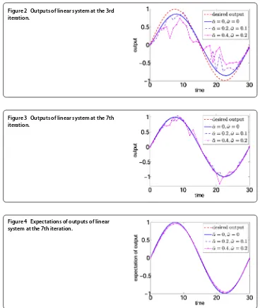
Figure 2 Outputs of linear system at the 3rd iteration.
Figure 3 Outputs of linear system at the 7th iteration.
Figure 4 Expectations of outputs of linear system at the 7th iteration.
The desired trajectory is chosen asyd(t) =sin(πt),t∈S. The beginning control signal is set
asu(t) = fort∈S–. For the proposed NILC scheme () with () and (), the convergent factor is computed asρ˜= –( –α¯)( – ω¯) under the assumption that the learning gain is restricted to∈(, ]. Thus, the convergent conditionρ˜< in Corollary holds if the probabilities satisfy ≤ ¯α< and ≤ ¯ω<, respectively.
Set the learning gain as= .. Choose three groups of probabilities as P:α¯= ,ω¯= ; P:α¯= .,ω¯= . and P:α¯= .,ω¯= ., respectively. It is testified that the convergent conditions for three groups of probabilities in Corollary areρ˜(P) = < ,ρ˜(P) =
,
, < andρ˜(P) = ,
,< , respectively, which implies that the convergent conditions are satisfied. Figures and depict the outputs for those three groups probabilities at the third and seventh iterations, respectively, where the dashed curves exhibit for the desired outputs, the solid ones denote the outputs for P:α¯= ,ω¯= , the dot-dash ones plot the outputs for P:α¯= .,ω¯= . and the circle-solid ones present the outputs for P:α¯= .,
¯
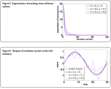
Figure 5 Expectations of tracking errors of linear system.
Figure 6 Outputs of nonlinear system at the 3rd iteration.
It is observed that the outputs for larger dropout probabilities render stronger stochastic oscillations and slower tracking. Figure displays the expectations of those outputs at the seventh iteration, while Figure shows the expectations of tracking errors, which convey that expectations of tracking errors with respect to the proposed NILC scheme () with () and () converge to nullity very well.
Example Consider a nonlinear system modeled as
x,k(t+ )
x,k(t+ )
=
sin(x,k(t))
cos(x,k(t))
+
uk(t), t∈S–={, , , . . . , },
yk(t) =x,k(t) +x,k(t), t∈S={, , , . . . , }, ()
x,k() = , x,k() = .
The desired trajectory is set asyd(t) =sin(πt),t∈S. The control signal at the beginning
iteration is set asu(t) = fort∈S–. It is calculated that the Lipschitz constant of the functionf(x,k(t),x,k(t)) = [sin(x,k(t)),cos(x,k(t))]isLf = . Under the assumption
that the learning gainis confined within the range (, ], the convergent factor is formu-lated asρ= –( –α¯)(. – ω¯). This means thatρ< holds if the probabilities are restricted as ≤ ¯α< and ≤ ¯ω< . are satisfied.
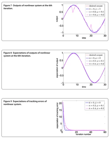
Figure 7 Outputs of nonlinear system at the 6th iteration.
Figure 8 Expectations of outputs of nonlinear system at the 6th iteration.
Figure 9 Expectations of tracking errors of nonlinear system.
desired outputs, the solid ones are the outputs for P:α¯ = , ω¯ = , the dot-dash ones express the outputs for P:α¯= .,ω¯= . and the circle-solid ones represent the outputs for P:α¯= .,ω¯= ., respectively.
It is seen that the outputs are closing to the desired trajectory as the iteration goes on, though the outputs for larger dropout probabilities reveal stochastic perturbation. Fig-ure plots the expectations of outputs at the sixth iteration on operation time interval, while Figure depicts the expectations of tracking errors along the iteration direction, respectively.
6 Conclusion
In this paper, a D-type NILC scheme is developed for discrete-time systems with appropri-ate mending manners for dropped input and output data. Under the assumption that the stochastic data dropouts are subject to - Bernoulli-type distributions and by assessing the tracking performance in the form of mathematical expectation, the zero-error con-vergences of the NILC for the SISO linear and affine nonlinear time-invariant systems are derived, respectively. Both the theoretical derivations and the numerical simulations con-vey that the proposed NILC scheme enables the linear and affine nonlinear time-invariant systems to track the desired trajectory well, though the stochastic dropout may disturb the tracking behavior. However, the investigations for the networked ILC systems with noise and parameter uncertainties are challenging in future work.
Competing interests
The authors declare that they have no competing interests.
Authors’ contributions
All authors contributed equally and significantly in writing this article. All authors read and approved the final manuscript.
Acknowledgements
The authors sincerely appreciate the support of the National Natural Science Foundation of China under granted No. F010114-60974140 and 61273135.
Received: 6 July 2016 Accepted: 2 February 2017
References
1. Arimoto, S, Kawamura, S, Miyazaki, F: Bettering operation of robots by learning. J. Robot. Syst.1(2), 123-140 (1984) 2. Bristow, DA, Tharayil, M, Alleyne, AG: A survey of iterative learning control. IEEE Control Syst. Mag.26(3), 96-114 (2006) 3. Chen, Y, Moore, KL, Yu, J, Zhang, T: Iterative learning control and repetitive control in hard disk drive industry - a
tutorial. Int. J. Adapt. Control Signal Process.22(4), 325-343 (2008)
4. Mi, CT, Lin, H, Zhang, Y: Iterative learning control of antilock braking of electric and hybrid vehicles. IEEE Trans. Veh. Technol.54(2), 486-494 (2005)
5. Chen, Y, Wen, C, Gong, Z, Sun, M: An iterative learning controller with initial state learning. IEEE Trans. Autom. Control 44(2), 371-376 (1999)
6. Park, KH, Bien, Z: Intervalized iterative learning control for monotonic convergence in the sense of sup-norm. Int. J. Control78(15), 1218-1227 (2005)
7. Ruan, XE, Wang, Q: Convergence properties of iterative learning control processes in the sense of the Lebesgue-P norm. Asian J. Control14(4), 1095-1107 (2012)
8. Bu, XH, Hou, ZS: Adaptive iterative learning control for linear systems with binary-valued observations. IEEE Trans. Neural Netw. Learn. Syst. (2016). doi:10.1109/TNNLS.2016.2616885.
9. Krtolica, R, Ozguner, U, Chan, H, Goktas, H, Winkelman, J, Liubakka, M: Stability of linear feedback-systems with random communication delays. Int. J. Control59(4), 925-953 (1994)
10. Yang, FW, Wang, ZD, Hung, YS, Gani, M: H-infinity control for networked systems with random communication delays. IEEE Trans. Autom. Control51(3), 511-518 (2006)
11. Wen, DL, Yang, GH: Dynamic output feedback H-infinity control for networked control systems with quantisation and random communication delays. Int. J. Syst. Sci.42(10), 1723-1734 (2011)
12. Wu, J, Chen, TW: Design of networked control systems with packet dropouts. IEEE Trans. Autom. Control52(7), 1314-1319 (2007)
13. Wang, D, Wang, JL, Wang, W: H-infinity controller design of networked control systems with Markov packet dropouts. IEEE Trans. Syst. Man Cybern. Syst.43(3), 689-697 (2013)
14. Liu, C, Xu, J, Wu, J: Iterative learning control for remote control systems with communication delay and data dropout. Math. Probl. Eng.2012, Article ID 705474 (2012)
15. Bu, XH, Yu, FS, Hou, ZS, Wang, FZ: Iterative learning control for a class of nonlinear systems with random packet losses. Nonlinear Anal., Real World Appl.14(1), 567-580 (2013)
16. Liu, J, Ruan, XE: Networked iterative learning control approach for nonlinear systems with random communication delay. Int. J. Syst. Sci.47(16), 3960-3969 (2016)
17. Ahn, HS, Chen, Y, Moore, KL: Intermittent iterative learning control. In: Proceedings of the 2006 IEEE International Conference on Intelligent Control, Munich, Germany, pp. 144-149 (2006)
18. Ahn, HS, Moore, KL, Chen, YQ: Discrete-time intermittent iterative learning control with independent data dropouts. In: Proceedings of 17th IFAC World Congress, Seoul, Korea, pp. 12442-12447 (2008)
19. Ahn, HS, Moore, KL, Chen, YQ: Stability of discrete-time iterative learning control with random data dropouts and delayed controlled signals in networked control systems. In: Int. Conf. Control., Autom., Robot. Vis., ICARCV Hanoi, Vietnam, pp. 757-762 (2008)
21. Bu, XH, Hou, ZS, Jin, ST, Chi, RH: An iterative learning control design approach for networked control systems with data dropouts. Int. J. Robust Nonlinear Control26(1), 91-109 (2016)
22. Bu, XH, Hou, ZS, Yu, FS, Wang, FZ: Hinf iterative learning controller design for a class of discrete-time systems with data dropouts. Int. J. Syst. Sci.45(9), 1902-1912 (2014)
23. Shen, D, Wang, YQ: Iterative learning control for networked stochastic systems with random packet losses. Int. J. Control88(5), 959-968 (2015)
24. Shen, D, Wang, YQ: ILC for networked nonlinear systems with unknown control direction through random lossy channel. Syst. Control Lett.77, 30-39 (2015)