A Metaheuristic Framework for Bi-level Programming Problems with Multi-disciplinary Applications

White Rose Research Online

[email protected]

Universities of Leeds, Sheffield and York

http://eprints.whiterose.ac.uk/

This is an author produced version of a paper published in

Studies in

Computational Intelligence.

White Rose Research Online URL for this paper:

http://eprints.whiterose.ac.uk/75425/

Published paper:

Koh, ATM (2013)

A Metaheuristic Framework for Bi-level Programming Problems

with Multi-disciplinary Applications.

In: Metaheuristics for Bi-level Optimization.

Studies in Computational Intelligence, 482 . Springer, Berlin, Heidelberg , 153 -

187 .

Programming Problems with MultiDisciplinary

Applications

Andrew Koh

Abstract Bi-level programming problems arise in situations when the decision

maker has to take into account the responses of the users to his decisions. Several problems arising in engineering and economics can be cast within the bi-level pro-gramming framework. The bi-level propro-gramming model is also known as a Stack-leberg or leader-follower game in which the leader chooses his variables so as to optimise his objective function, taking into account the response of the follower(s) who separately optimise their own objectives, treating the leader’s decisions as ex-ogenous. In this chapter, we present a unified framework fully consistent with the Stackleberg paradigm of bi-level programming that allows for the integration of meta-heuristic algorithms with traditional gradient based optimisation algorithms for the solution of bi-level programming problems. In particular we employ Differ-ential Evolution as the main meta-heuristic in our proposal. We subsequently apply the proposed method (DEBLP) to a range of problems from many fields such as transportation systems management, parameter estimation and game theory. It is demonstrated that DEBLP is a robust and powerful search heuristic for this class of problems characterised by non smoothness and non convexity.

1 Introduction

This paper introduces a meta-heuristic framework for solving the Bi-level program-ming Problem (BLPP) with a multitude of applications [26, 74]. As a historical footnote, the term “bi-level programming” was first coined in a technical report by Candler and Norton in [20] who were concerned with general multilevel program-ming problems. The BLPP is a special case of a multilevel programprogram-ming problem restricted to two levels. Prior to that time, the BLPP was known simply as a

math-Andrew Koh

Institute for Transport Studies, University of Leeds, Leeds, LS2 9JT, United Kingdom e-mail:

[email protected]

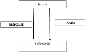
ematical program with an optimisation problem in the constraints [18] but had al-ready found military applications [19]. In economics and game theory, a BLPP is a Stackleberg [106] or “leader-follower” game (see Fig. 1) in which the leader chooses his variables so as to optimise his objective but continues to take into account the response of the follower(s) who when independently optimising their separate ob-jectives, treat the leader’s decisions as an exogenous input [72].

Fig. 1 Pictoral Representation of a BLPP

BLPPs possess in common the following three characteristics [86, 117]:

• The decision-making units are interactive and exist within a hierarchical struc-ture.

• Decision making is sequential from higher to lower level. The lower level deci-sion maker executes its policies after decideci-sions are made at the upper level.

• Each unit independently optimises its own objective functions but is influenced by actions taken by other units.

The BLPP has been a subject of intense research and several notable volumes have been published to date [7, 32, 72, 87]. At the same time applications of BLPP can be found in fields as diverse as chemical engineering [49], robot motion planning and control [72], production planning [8] occurring in a multitude of disciplines [7]. In tandem, there has been much work on the development of solution methodologies (see [26, 32] for a review of these).

2 The Bi-Level Programming Problem

2.1 A General BLPP

We can write a generic BLPP as the system of equations in Eq. 1. The unique feature of Eq. 1 is that the constraint region is implicitly determined by yet another optimi-sation problem1. This constraint is always active. The upper level problem denoted as Program U, is given in Eq. 1a,

Program U

      

min

x∈XU(x,y) subject to

G(x,y)≤0

E(x,y) =0

(1a)

where for given x, y is the solution to the lower level program (Program L) in 1b:

Program L

        

min

y∈YL(x,y) subject to

g(x,y))≤0

e(x,y)) =0

(1b)

In the formulation in Eq. 1 we define the following mappings: U,L :Rn1_×Rn2_→

R1_{,G :R}n1_×Rn2_→Rq1_{, g :R}n1_×Rn2_→Rq2_{, E :R}n1_×Rn2_→Rr1_{, e :R}n1_×Rn2_→

Rr2_{. In the general case the objectives and constraints at both levels are non-linear.}

The sets X and Y representing the search domains for 1a and 1b respectively are defined as follows: X =

(x1,x2, ....,xn1)

⊺_∈ Rn1_xl

i≤xi≤xui ,i=1, ...,n1 and Y =n(y1,y2, ....,yn2)

⊺_∈ Rn2

y

l

j≤yj≤yuj,j=1, ...,n2

o

with⊺denoting the

transpose. Arising from the “leader-follower” analogy of BLPPs, we use the terms leader’s variables and upper level variables interchangeably when referring to x.

2.2 Mathematical Programs with Equilibrium Constraints

We also define a class of BLPPs known as the Mathematical Programs with Equi-librium Constraints (MPECs). MPECs are BLPPs where the lower level problem consists of a variational inequality (VI) [26].

1_{Hence the original name of mathematical programs with optimisation problems in the constraints}

Program U

      

min

x∈XU(x,y) subject to

G(x,y)≤0

E(x,y) =0

(2a)

where for given x, y is the solution of the VI in Program L 2b:

L(x,y)⊺_(y−y∗_{)≥0,∀y∈}ϒ_{(x) (2b)}

Another class of problems closely related to MPECs are Mathematical Programs with Complementarity Constraints [67] which feature in place of a VI, a Comple-mentarity Problem instead in Program L. However since the VI is a generalization of the Complementarity Problem [56, 82], we will treat these two categories as syn-onymous for the purposes of this chapter and neglect the theoretical distinctions. We return in Section 4 to give an example of MPECs that arise naturally in transporta-tion systems management.

2.3 Solution Algorithms for the BLPP

When all functions (both objectives and constraints) at both levels are linear and affine, this class of problems is known as the linear-BLPP. However even in this de-ceptively “simple” case the problem is still nondeterministic polynomial time hard [11]. Even when both the upper level and the lower level are convex programming problems, the resulting BLPP itself can be non-convex [12]. Non convexity sug-gests the possibility of multiple local optima. Ben-Ayed and Blair [11] demonstrated the failure of both the Parametric Complementarity Pivot Algorithm [13] and the Grid Search Algorithm [5] to locate the optimal solution. Since then, progress has been made in solving the linear-BLPP and techniques including implicit enumera-tion [21], penalty based methods [2] and methods based on Karush -Kuhn-Tucker (KKT) conditions [41] have been developed. (See [117] for a detailed review of the algorithms available for the linear-BLPP).

Turning to solution algorithms for the general BLPP, several intriguing attempts have been proposed to solve it. One early proposal was the Iterative Optimisation Algorithm (IOA) [3, 107]. This method involved solving the Program U for fixed y and using the solution thus obtained to solve the lower level problem, Program L, and repeatedly iterating between the two programs until some convergence criteria is met. However the IOA was shown to be an exact method for solving a Cournot Nash game [40, 42] rather than the Stackleberg game that the BLPP reflects. The IOA implicitly assumes that the leader is myopic as he does not take into account the follower’s reaction to his policy [42]. To be consistent with the Stackleberg model, the leader must be modelled as endowed with knowledge of the follower’s reaction function which the leader knows the follower will obey.

The penalty interior point algorithm (PIPA) was proposed in [72]. Unfortunately a counterexample in [67] demonstrates that PIPA can converge to a nonstationary point. Subsequent research has led to the development of many other techniques to solve the MPEC such as the piecewise sequential quadratic programming in [72], branch-and-bound [6], nonsmooth approaches [32, 87] and smoothing methods [38]. Wrapping up this section, we summarise briefly the use of methods based on meta-heuristics. Meta-heuristics including stochastic optimisation techniques are recognised as useful tools for solving problems such as the BLPPs which do not necessarily satisfy the classical optimisation assumptions of continuity, convex-ity and differentiabilconvex-ity. Techniques include Simulated Annealing (SA) [1], Tabu Search (TS) [48], Genetic Algorithms (GA) [47], Ant Colony Optimisation (ACO) [34], Particle Swam Optimisation (PSO) [57] and Differential Evolution (DE) [94, 95, 108].

SA was used to optimise a chemical process plant layout design problem formu-lated as a BLPP in [101] and a Network Design Problem formuformu-lated as an MPEC [43]. ACO techniques for BLPPs are found in [93]. GAs have been used to solve BLPPs in inter alia [73, 86, 111, 114, 122]. PSO was applied to BLPPs in e.g. [126]. DE was used for BLPPs in [61] where an example demonstrated the inability of the TS method implemented in [96] to locate the global optima of a test func-tion. Despite their reported successes in tackling very difficult problems, it must be emphasised that heuristics provide no guarantee of convergence to even a local optimum. Despite this heuristics have been succesfully used to solve a variety of difficult problems such as the BLPP.

3 Differential Evolution for Bi-Level Programming (DEBLP)

Differential Evolution for Bi-Level Programming (DEBLP) was initially proposed in [61] to tackle BLPPs arising in transportation systems management. It is devel-oped from the GA Based Approach proposed in [111, 122] but substitutes the use of binary coded GA strings with real coded DE [95] as the meta-heuristic instead.

DE is a simple algorithm that utilises perturbation and recombination to optimise multi-modal functions and has already shown remarkable success when applied to the optimisation of numerous practical engineering problems [94, 95, 108]. On the other hand, many years of research have resulted in the development of a plethora of robust gradient based algorithms for tackling many operations research questions posed as non-linear programming problems (NLP) [9, 70, 85]. If we momentarily ignore the upper level problem, then for fixed x, Eq. 1b is effectively an NLP2which can be tackled by dedicated NLP tools such as sequential quadratic programming [9, 70, 85]. Such considerations motivated the development of the DEBLP meta-heuristic which sought to synergise DE’s well-documented global search capability to optimise the upper level problem with the dedicated NLP tools focused on solving

2_{Note that for fixed x, the lower level problem in the MPEC in Eq. 2b can also be solved using}

the lower level problem. More importantly, as we shall emphasise later, DEBLP continues to maintain the crucial “leader-follower” paradigm upon which the BLPP is founded.

In the rest of this section, we provide an overview of the operation of the DEBLP algorithm and discuss some of its limitations. However we temporarily neglect con-sideration of the q1+r1upper level constraints in Program U . Our discussion of the procedure used to ensure satisfaction of the upper level inequality and/or equality constraints is postponed till later (see Section 6).

3.1 Differential Evolution

Conventional deterministic optimisation methods generally operate on a single trial point, transforming it using search directions computed based on first (and possibly, second) order conditions until some criteria measuring convergence to a stationary point is satisfied [9, 70, 85]. On the other hand, population based meta-heuristics such as DE operate with a population of trial points instead. The idea here is that of improving each member throughout the operation of the algorithm by way of an analogy with Darwin’s theory of evolution3_.

Let there be π members in such a population of trial points. Specifically we denote the population at iteration it as Pit. An illustration of such a popula-tion is given in Eq. 3. Each member of Pit representing a single trial point

xit_k = (xit_k,1, . . . ,xit_k,n

1),k={1, . . . ,π}, also known as an individual, is a n1

dimen-sional vector that represents the upper level variables (see Eq. 1a). To avoid nota-tional clutter, we drop the it superscript as long as it does not lead to confusion. Without loss of generality, we will assume minimization. The DEBLP algorithm is outlined in Algorithm 1 which we elaborate upon in the ensuing paragraphs of this section.

Pit₌        

xit₁

.. .

xit_k

.. . xit π         =        

xit_1,1 xit_1,2· · · xit_1,n

1

..

. ... . .. ...

xit_k,1 xit_k,2 · · · x_kit_,n

1

..

. ... . .. ...

xit_π,1xit_π,2· · · xit_π,n

1         (3)

3_{Hence some of these methods are sometimes referred to as evolutionary algorithms in the}

Algorithm 1 Differential Evolution for Bi-Level Programming (DEBLP)

1. Randomly generate parent populationPofπindividuals. 2. EvaluateP

set iteration counter it=1

3. While stopping criterion not met, do: For each individual inPit_{, do:}

(a) Mutation and Crossover to create a single child from individual. (b) Evaluate the child using a hierarchical strategy.

(c) Selection: If the child is fitter than the individual, the child replaces the parent. Otherwise, the child is discarded.

End For

it=it+1 End While

3.1.1 Generate Parent Population

When the algorithm begins, real parameters in each dimension i of each member k ofP_{, that comprise the parent population, are randomly generated within the lower}

and upper bounds of the domain of the BLPP as in Eq. 4.

xk,i=rand(0,1)(xui −xli) +xli,k∈ {1, ...,π},i∈ {1, ...,n1}. (4) In Eq. 4 rand(0,1)is a pseudo random number generated from an uniform dis-tribution between 0 and 1.

3.1.2 Evaluation

The evaluation process to determine the fitness4of a trial point in the population has to be developed within the Stackleberg model [106] since we have to specifically model the leaders taking into account the response (reaction) of the followers to his strategy x. One way to accomplish this is via a “two stage” or hierarchical strategy which is achieved as follows.

In the first stage, for each individual k vector of the leader’s decision variables

xk, we solve Program L i.e. Eq. 1b to obtain y by using deterministic methods such as linear programming or sequential quadratic programming [9, 70, 85]. With y so obtained, we are then able to carry out the second stage which involves computing the value of the upper level objective U , corresponding to each individual vector of the leader’s decision variables input in the first stage.

It is worth highlighting that this procedure is different from the IOA described earlier in Section 2 as DEBLP obviates any iteration between the two levels. Instead, entirely consistent with the “leader-follower” paradigm, the leader’s vector xkbeing

4_{The term “fitness” used in such evolutionary meta-heuristics is borrowed from its analogy with}

manipulated by DE is offered as an exogenous input to the lower level program to be solved in the first stage. One obvious drawback of doing this is the resulting increase in computational burden which has been significantly reduced by advances in computing power.

3.1.3 Mutation and Crossover

The objective of mutation and crossover is to produce a child vector wkfrom the parent. This is accomplished by stochastically adding to the parent vector the fac-tored difference of two other randomly chosen vectors from the population as shown in Eq. 5.

wk,i=

xs1,i+λ(xs2,i−xs3,i)

xk,i

if rand(0,1)<χor i=intr(1,n1)

otherwise (5)

In Eq. 5, s1,s2 and s3∈ {1,2, . . . ,π} are randomly chosen population indices distinct from each other and also distinct from the current population member in-dex k. rand(0,1)is a pseudo random real number between 0 and 1 and intr(1,n1) is a pseudo random integer between 1 and n1. The mutation factorλ ∈(0,2)is a parameter which controls the magnitude of the perturbation andχ∈[0,1]is a prob-ability that controls the ratio of new components in the offspring. The or condition in Eq. 5 ensures that the child vector wkwill differ from its parent xkin at least one dimension.

We stress that the mutation and crossover strategy shown in Eq. 5 is not the only possible strategy available though this is the one used in this work. Other strategies are found in [94, 95, 108]. Nevertheless all the strategies of DE reflect a common theme: the creation of the child vector wkvia the arithmetic recombination of ran-domly chosen vectors along with addition of difference vector(s) typified in Eq. 5.

3.1.4 Enforce Bound Constraints

Mutation and crossover can however produce child vectors that lie outside the bounds of the original problem specification. There are several ways to ensure satis-faction of these constraints. One could set the parameter equal to the limit exceeded or regenerate it within the bounds. Alternatively, following [94], we reset out of bound values in each dimension i half way between its pre-mutation value and the bound violated as shown in Eq. 6.

w_k,i=

    

xk,i+xli

2 if wk,i<xli xk,i+xui

2 if wk,i>xui

w_k,iotherwise

3.1.5 Selection

Once the hierarchical evaluation process is carried out on the child vector w_k pro-duced, we can compare the fitness obtained with that of its parent x_k. This means that comparison is against the same k parent vector5_{on the basis of whichever of} the two gives a lower value for Program U . Assuming minimization the one that produces a lower value survives to become a parent in the following generation as shown in Eq. 7.

xit_k+1 =

wit_k xit_k

if U(wit_k,L(•))≤U(xt_k,L(•))

otherwise (7)

These steps are repeated until some user specified termination criteria is met, and this is usually when it reaches the maximum number of iterations, although other criteria are possible [95].

3.2 Control Parameters of DE

Unless otherwise stated, for all experiments reported throughout this chapter we used a Mutation Factor, λ, of 0.9 and a Probability of Crossover,χ, of 0.9. The population size,π, and the maximum number of iterations allowed varied for each of the BLPPs we investigated and these will be clearly stated in the relevant sections. Because DEBLP is a stochastic meta-heuristic, we always carry out 30 independent runs with different random seeds. All numerical experiments were conducted using MATLABTM7.8 running on a 32 bit WindowsTMXP machine with 4 GB of RAM.

3.3 Implicit Assumptions of DEBLP

Through the rest of this paper we will demonstrate in examples from various dis-ciplines that DEBLP is a powerful and robust solution methodology for handling a variety of problems formulated as BLPPs. However we are cognizant at the outset two key limitations of our approach:

1. DEBLP is a heuristic: with its strength arising from it avoiding reliance on the ob-jective functions being differentiable and/or satisfying convexity properties and hence able to handle a large class of intrinsically non smooth problems. How-ever it should recognised that for this very reason, it is not generally possible to establish convergence of the algorithm to even a local optimum.

2. DEBLP implicitly assumes that the Program L is convex for fixed x and can be solved to global optimality by deterministic methods and that failure to solve the

lower level problem to global optimality does not affect the solution of Program

U .

This section has focused on defining the motivation for, and outlining, the DE-BLP meta-heuristic which sought to synergise the exploratory power of DE with robust deterministic algorithms focused on solving the lower level problem. Rec-ognizing its limitations, in the next section, we apply DEBLP to control problems arising from Transportation Systems Management formulated as BLPPs where the lower level program is shown to be convex for a given tuple of the leader’s variables.

4 Applications to Transportation Systems Management

In this section, we study two problems in transportation systems management. In applications, the leader in Program U could be thought of as a regulatory authority applying control strategies (policy) that influence the travel choices of the followers who are the highway users on the road network. It will be shown under certain assumptions, the followers problem can be established as a VI thus the problems under consideration are MPECs.

4.1 The Lower Level Program in Transportation

In the transportation systems management literature, Program L has an interpre-tation in that it is the mathematical formulation representing the follower’s (road user’s) route choice [15] on a highway network. This is often referred to as the Traf-fic Assignment Problem (TAP). TrafTraf-fic assignment aims to determine the number of vehicles and the travel time on different road sections of a traffic network, given the travel demand between different pairs of origins and destinations [60].

Definition 1 [115] The journey times on all the routes actually used are equal, and

not greater than those which would be experienced by a single vehicle on any unused route.

The TAP is founded on the behavioral premise of Wardrop’s User Equilibrium as given in Definition 1. In effect this states that user equilibrium is attained when no user can decrease his travel costs by unilaterally changing routes. The TAP provides the link flow vector (v) when user equilibrium is attained.

To facilitate exposition of Program L, consider a transportation network repre-sented as a graph with N nodes and A links/arcs, and let:

P: the set of all paths/routes in the network,

H: the set of all Origin Destination (OD) pairs in the network, Ph: the set of paths connecting an OD pair h,h∈H,

va: the link flow on link a v= [va],a∈A,

ca(va): the travel cost of utilising the link a, as a function of link flow vaon that link only, c(v) = [ca(va)],a∈A

cp: the travel cost of path p,p∈P,

δap: a dummy variable that is 1 if the path p,p∈P uses link a ,a∈A, 0 otherwise and

Ω: the set of feasible flows and demands.

On the demand side, we assume that there is an amount of demand dh,h∈H (dh≥0) wishing to travel between OD pair h andµhis the minimum travel cost that OD pair h,h∈H.

4.1.1 TAP as a Variational Inequality

Lemma 1. Wardrop’s Equilibrium Condition of route choice implies that at

equilib-rium the following conditions are simultaneously satisfied: Fp∈Ph ≥0⇔cp∈Ph=µh ∀h∈H,∀p∈P;

Fp∈Ph =0⇔cp∈Ph≥µh ∀h∈H,∀p∈P;

d_h= ∑

p∈Ph

Fp ∀h∈H,∀p∈P;

Lemma 1 states that path p connecting OD pair h will be used by the travellers if and only if the cost of travelling on this route is the minimum travel cost between that OD pair. The Variational Inequality (VI) in Eq. 8 restates Wardrop’s Equilib-rium Condition.

Find v∗∈Ω such that c(v∗)⊺_(v−v∗_{)≥0,∀v∈}Ω ₍₈₎

Proposition 1. The solution of the Variational Inequality defined in Eq. 8 results

in a vector of link flows demands (v∗∈Ω)that satisfies Wardrop’s Equilibrium Condition of route choice given by Lemma 1.

Proof. For a proof of Proposition 1, see [28, 105]. ⊓⊔

4.1.2 Convex Optimisation Reformulation

In the particular instance (and in the cases considered in this chapter) when the travel cost of using a link is dependent only on its own flow6, there exists an equivalent convex optimisation program for the VI (Eq. 8) as shown in Eq. 9.

min

v L=

∑

∀a

va

Z

0

c_a(z)dz (9a)

Subject to:

∑

p∈Ph

Fp=dh,h∈H (9b)

va=

∑

Fpδap,a∈A (9c)

Fp≥0,p∈P. (9d)

The objective of the program in Eq. 9 is a mathematical construct, with no be-havioral interpretation, employed to solve for the equilibrium link flows that satisfies Wardrop’s Equilibrium Condition [103]. In this program, the first constraint states that the flow on each route used by each OD pair is equal to the total demand for that OD pair. The second constraint is a definitional constraint which stipulates that the flow on a link comprises flow on all routes that use that link. The last constraint restricts the equilibrium flows and demands to be non negative. These linear con-straints defineΩ. SinceΩ is closed and convex, the equilibrium link flows v∗∈Ω

are unique [15]. In practice, it is usually the case that traffic assignment algorithms (see examples in texts such as [89, 103]) are used to solve Program L.

4.2 Continuous Optimal Toll Pricing Problem (COTP)

The continuous optimal toll pricing problem involves selecting an optimal toll level for each predefined tolled link in the network [11]. With a view to controlling con-gestion, there has been renewed interests by transportation authorities globally to study this “road pricing ” problem (e.g. Singapore, London, Stockholm).

4.2.1 Model Formulation

In addition to the notation defined at the start of this section, we introduce the fol-lowing notation to describe the COTP. Let:

ta(va): the travel time on link a, as a function of link flow vaon that link only,

T : the set of links that are tolled T⊆A

τ: the vector of tolls,τ= [τa], a∈T

τmax

a ,τamin: the upper and lower bounds of toll charge on link a, a∈T

min

τ U=

∑

a∈A

vata(va) (10a)

Subject to:

τmin

a ≤τa≤τamax, a∈T

τa=0, a∈/T

(10b)

Note however that v can only be obtained by solving Program L in Eq. 9. Thus in terms of Figure 1, the policy variables x is the toll vector τ and the follower’s response is the traffic routing that manifests in the vector of link flows on the road network v that in turns affect the leader’s objective.

Recall that in defining the lower level program in Eq. 9, the road user was as-sumed to consider the travel cost of utilising an arc a, a∈A. Eq. 11 maps the travel

time ta(va)on an arc a, into the equivalent travel costs ca(va).

ca(va) =

ta(va) +τa

ta(va)

if a∈T

otherwise (11)

4.2.2 Previous Work on the COTP

Various solution algorithms have been proposed for the COTP. Yang and Lam pro-posed a linearisation based method that uses derivative information to form approx-imations to the upper level objective [118] known as a sensitivity based analysis algorithm (SAB). However it has been pointed out [122] the global optimality of the SAB algorithm is not assured and that obtaining a local optimum is indeed pos-sible. Another derivative-based method was derived from constraint accumulation [66]. A review of algorithms for the COTP is found in [111].

4.2.3 Example

We illustrate the use of DEBLP to solve the COTP with an example from [118]. Fig. 2 shows the network which has 6 nodes and 7 links. Link numbers are written above the links and node numbers are indicated accordingly. There are two OD pairs between nodes 1 and 3 and between 2 and 4 of 30 trips each. The rest of the nodes represent junction/intersections of the road network and travel is in the direction indicated by the arrows. The link travel times ta(va)take the explicit function forms as given in Eq. 12.

ta(va) =ta0(1+0.15(

va

Capa

)4_{) (12)}

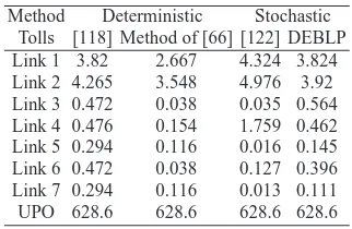
For this example, we use a population size,π, of 20 and allowed a maximum of 50 iterations in each of 30 runs. Table 2 compares the results of DEBLP with that of two deterministic algorithms (direct from [118] and our implementation of the algorithm of [66] together with a GA based method from [122]. UPO refers to the value of (Upper level) Objective in Eq. 10. It can be seen from Table 2 that the four different algorithms provided different tolls underlying the multimodal nature of this problem. However the upper level objective function values are the same in all cases. This bears testimony to the multimodal nature of the COTP where many different toll vector tuples could potentially result in attaining the same upper level objective function value.

Table 1 Network Parameters for COTP Example

Link a t0

aCapaτamax

1 8 20 5 2 9 20 5 3 2 20 2 4 6 40 2 5 3 20 2 6 3 25 2 7 4 25 2

Table 2 Comparison of existing against DEBLP

results for COTP Example

Method Deterministic Stochastic Tolls [118] Method of [66] [122] DEBLP Link 1 3.82 2.667 4.324 3.824 Link 2 4.265 3.548 4.976 3.92 Link 3 0.472 0.038 0.035 0.564 Link 4 0.476 0.154 1.759 0.462 Link 5 0.294 0.116 0.016 0.145 Link 6 0.472 0.038 0.127 0.396 Link 7 0.294 0.116 0.013 0.111 UPO 628.6 628.6 628.6 628.6

Fig. 2 Network for COTP Example [118] Fig. 3 Network for CNDP Example 1 [27]

4.3 Continuous Network Design Problem

4.3.1 Model Formulation

To proceed with this example, we introduce additional notation as follows (others as previously defined):

κ: the set of links that have their individual capacities enhanced,κ⊆A.

β: the vector of capacity enhancements,β= [βa], a∈κ

βmax

a ,βamin: the upper and lower bounds of capacity enhancements, a∈κ.

da: the monetary cost of capacity increments per unit of enhancement, a∈κ.

Cap0_a: existing capacity of link a, a∈A.

θ: conversion factor from monetary investment costs to travel cost units. In the CNDP, the regulator aims to minimise the sum of the total travel times and investment costs with constraints on the amount of capacity additions while Program

L determines the user’s route choice, for a givenβ, once again based on Wardrop’s principle of route choice as mentioned previously. Hence the CNDP seeks a |κ|

dimension vector of capacity enhancements optimal to the following BLPP in Eq. 13:

min

τ U=

∑

a∈A

vata(va) +

∑

∀a∈K

θdaβa (13a)

subject to:

βmin

a ≤βa≤βamax a∈κ;

βa=0 a∈/κ

(13b)

where v is the solution of a lower level TAP (Program L) Eq. 9, parameterised in the vector of capacity enhancements for the fixed demand case. We map the travel times to the travel costs by means of Eq. 14.

ca(va) =

(

t0

a(1+0.15(Capv0a

a+βa)

4₎

t0

a(1+0.15(Capva0

a)

4₎

if a∈κ

if a∈/κ (14)

4.3.2 Previous Work on CNDP

4.3.3 Example 1: Hypothetical Network

The network for the first example is taken from [27] and reproduced in Fig. 3. This network has 6 nodes and 2 OD pairs; the first between nodes 1 and 6 of 10 trips and the second, between nodes 6 and 1 of 20 trips. Please refer to [27] for the link parameter details. Note thatβmin

a =0 andβ max

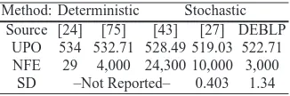
a = 20,∀a∈κ,κ⊆A as in [27]. We assumed a population size,π, of 20 and allowed a maximum of 150 iterations. Table 3 summarises the results that have been reported previously and compares it with the results reported in our paper. UPO refers to the value of (upper level) objective in Eq. 13. NFE is the number of function evaluations. Note that the number of lower level programs solved equal to population size multiplied by the maximum number of iterations allowed. SD is the standard deviation over 30 runs. Our results are based on the mean of these 30 runs. Though the SD of the GA method is much lower, [27] also reported using local search method to aid the search process which accounts for the higher NFE as well.

4.3.4 Example 2: Sioux Falls Network

The second example is the CNDP for the Sioux Falls (South Dakota,USA) network with 24 nodes, 76 links and 552 OD pairs. The network parameters and OD details are found in [75]. Only 10 links out of the 76 are subject to improvements.

While this network is clearly larger and arguably more realistic, the problem dimension (i.e. leader’s variables simultaneously optimised) is smaller than in Ex-ample 1, since 10 links are subject to improvement rather than the 16 links in the former. This offers an explanation as to why the number of function evaluations (NFE) reported in all studies compared is less than for the first example. The re-sults are compared in Table 4. Our rere-sults show the mean of 30 runs with different random seeds.

It can be deduced from Table 4 that DEBLP is able to locate the global optimum; again with a lesser number of iterations than the SA method in [43]. More inter-estingly, DEBLP required less iterations than the deterministic method of [75]. The standard deviation is also very low which suggests that this heuristic is reasonably robust as well.

Table 3 Comparison of existing against DEBLP

results for CNDP Example 1

Method: Deterministic Stochastic Source [24] [75] [43] [27] DEBLP

UPO 534 532.71 528.49 519.03 522.71 NFE 29 4,000 24,300 10,000 3,000

SD –Not Reported– 0.403 1.34

Table 4 Comparison of existing against DEBLP

results for CNDP Example 2

Method: Deterministic Stochastic Source [24] [75] [43] DEBLP

5 Applications to Parameter Estimation Problems

In this section we derive the Error-In-Variables model and show that it can be for-mulated as a BLPP and apply it to 2 examples from [49]. Parameter estimation is an important step in the verification and utilization of mathematical models in many fields of science and engineering [37, 49, 59]. In the classical least-squares approach to parameter estimation, it is implicitly assumed that the set of independent variables is not subject to measurement errors [46]. On the other hand, the error-in-variables (EIV) approach assumes that there are measurement errors in all variables [16, 98].

5.1 Formulation of EIV Model

We consider models of the implicit form as in Eq. 15.

f(x,y) =0 (15) In Eq. 15, x is the vector of n1unknown parameters, y is the vector of n2 measure-ment variables and f is the system of algebraic functions. The measured variables are the sum of the true valuesζmwhich are unknown and the additive error termεm at the data point m as shown in Eq. 16.

ym=ζm+εm (16) We assume that the error is normally distributed with zero mean and possessing a known covariance matrix. The vector of unknown parameters x can be estimated from the solution of the constrained optimisation problem in Eq. 17.

min ˆ x,yˆ

M

∑

m=1

(ˆym−ym)⊺Λ−1(ˆym−ym)

subject to

f(ˆy_m,xˆ) =0,m=1, . . . ,M

(17)

As mentioned, we do not know the true values ofζm. However they are approxi-mated from the optimisation as the fitted variables ˆy_m. Assuming that the covariance matrixΛis the same in each experiment and diagonal, we write Eq. 17 as Eq. 18.

min ˆ x,yˆ

M

∑

m=1 n2

∑

i=1

(yˆm,i−ym,i)2 σ2

i

subject to

f(ˆy_m,xˆ) =0,m=1, . . . ,M

(18)

Program U min ˆ x M ∑

m=1 n2

∑

i=1

(yˆm,i−ym,i)2 σ2

i

(19a)

where for given x, y is the solution to the lower level program (Program L):

Program L        min ˆ x,yˆ

M

∑

m=1 n2

∑

i=1

(yˆm,i−ym,i) σ2

i

subject to

f(yˆm,i,xˆ) =0,m=1, . . . ,M,i=1, . . . ,n2

(19b)

For a survey of the alternative optimisation based formulations of the EIV model, the reader is referred to [59].

5.2 Examples

We present 2 examples of the EIV model that were solved using deterministic meth-ods in the cited references. Note that we consider only a single common variance term for all variables and we can eliminate it from further consideration. In all our experiments of DEBLP we assumed a population size,π, of 20 and allowed a max-imum of 100 iterations.

5.2.1 Example 1: “Kowalik Problem”

Consider the model due to Moore et al in [76] known as the “Kowalik Problem” where we estimate the equation of the form in Eq. 20.

ˆ

ym,1=

x1y2_m,2+x1x2ym,2

y2

m,2+ym,2x3+x4

(20)

We have 11 data points for this model (see [49] for the data set). It is assumed that ym,1contains errors, and ym,2is error-free. The resulting BLPP is shown in Eq. 21. Notice that the lower level equality constraint in Eq. 21 is the model formulation hypothesised in Eq. 20.

min ˆ x

11

∑

m=1

(yˆm,1−ym,1)2 subject to

min

y

11

∑

m=1

(yˆm,1−ym,1)2 ˆ

ym,1(y2_m,2+ym,2x3+x4)−x1y2_m,2−x1x2ym,2=0

(21)

variables x1,x2,x3and x4. Table 5 shows the results which clearly agrees with that reported in [49]. In this table UPO refers to the objective of the upper level in Eq. 21. Note that the standard deviation of the UPO over the 30 independent DEBLP runs conducted was less than 1×10−5_.

5.2.2 Example 2: “Linear Fit”

The model we intend to estimate is a linear equation of the form in Eq. 22. The 10 data points are from [49]. Compared to Example 1, here we assume that measure-ment errors are present in both ym,1and ym,2, m={1, . . . ,10}.

ˆ

ym,2=x1+x2yˆm,1 (22) Assuming a common variance for each data tuple{ym,1,ym,2}, we can estimate the vector of unknown x parameters via the BLPP in Eq. 23.

min ˆ x

10

∑

m=1 2

∑

i=1

(yˆm,i−ym,i)2 subject to

min

y

10

∑

m=1 2

∑

i=1

(yˆm,i−ym,i)2 ˆ

ym,2−x1−x2yˆm,1=0

(23)

The results of 30 runs of DEBLP (with a maximum of 100 iterations allowed per run and a population sizeπ of 20) for this problem are shown in Table 6. Again the standard deviation over the 30 runs was less than 1×10−5. As with Example 1, the results obtained by DEBLP agrees with those reported in [49].

Table 5 Parameter Estimation Example 1 (“Kowalik Problem”)

Variable DEBLP [49]

x1 0.1928 0.1928

x2 0.1909 0.1909

x3 0.1231 0.1231

x4 0.1358 0.1358

UPO 0.000307 0.000307

Table 6 Parameter Estimation Example 2

(“Lin-ear Fit”)

Variable DEBLP [49]

x1 5.7840 5.784

x2 -0.544556 -0.54556

UPO 0.61857 0.61857

6 Handling Upper Level Constraints

and described a technique to ensure that the population remains within the search domain which was sufficient for the problem examples investigated. Before pro-ceeding to our next application area for BLPPs, we outline in this section, necessary modifications to DEBLP to enable it to handle them effectively.

6.1 Overview of Constraint Handling Techniques with

Meta-Heuristics

In their most basic form, meta-heuristics do not have the capability to handle gen-eral constraints aside from bound constraints. However since real world problems generally have linear and nonlinear constraints, a large amount of research effort has been expended on the topic of constraint handling with such algorithms. In the past few years many techniques have been proposed. Among others these include penalty methods [121], adaptive techniques [104], techniques based on multiobjec-tive optimisation [25, 65] etc.

The penalty method transforms the constrained problem into an unconstrained one. However one of the drawbacks of this method when applied with meta-heuristics is that the solution quality is sensitive to the penalty parameter used. The penalty parameter itself is problem dependent [99]. This method also encounters difficulties when solutions lie at the boundary of the feasible and infeasible space.

Recall the selection criteria of the DEBLP in Algorithm 1. In the presence of constraints, when we are deciding whether to accept or reject the child, wk, it is no longer a case of comparing the values of objective U attained. The key consideration is how one would say, decide between a infeasible individual with low U and a feasible individual but higher U .

Intuitively one could conclude that a feasible individual is better than the infea-sible individual because the aim is to ultimately seek solutions that minimise the objective function and satisfy all the constraints. This viewpoint however ignores the fact that the meta-heuristics are generally stochastic by design. There exists the possibility that the infeasible individuals could in fact be better than the feasible one at some iterations during the algorithm [124]. The question then is how to strike the right balance between objective and constraints.

6.2 Stochastic Ranking

Runarsson and Yao [99, 100] proposed an alternative constraint handling method known as stochastic ranking (SR)7to aid in answering this question. To use SR, the first step is to obtain a measure of the constraint violation, v(xk), of vector xkusing

Eqn. 24. The first term on the RHS of Eq. 24 sums the maximum of either 0 or the value of the inequality constraint Gj(xk),j∈ {1, . . . ,q1}8. The second term sums the absolute value of each of the equality constraints Ej(xk),j∈ {1, . . . ,r1}.

v(xk) = q1

∑

j=1

max{0,Gj(xk)}+ r1

∑

j=1

E_j(x_k)

(24)

The key operation of SR involves counting how many comparisons of adjacent pairs of solutions are dominated by the objective function and constraint violations. This is accomplished in SR through a stochastic bubble sort like procedure that is used to rank9_{the population. This comparison is illustrated in Algorithm 2 where}

rand(0,1)is a pseudo random real number between 0 and 1. The method requires a probability factorηwhich should be less than 0.5 to create a bias against infeasible solutions [99].

Suppose we have two individuals xk1 and xk2,k16=k2. If both do not violate constraints or if a pseudo random real number is less than or equal toη, we swap their rank order based on the objective function obtained, with the lower one be-ing assigned a higher rank. Otherwise we swap their ranks based on the constraint violations, again with the lower constraint violation being assigned a higher rank. Working our way through the population to be ranked, we continue comparing ad-jacent members according to Algorithm 2 and swapping ranks. When no change in rank order occurs, SR terminates.

Algorithm 2 Stochastic Ranking

if v(xk1) =0 and v(xk2) =0 or rand(0,1)≤η then

rank based on objective function value only

else

rank based on constraint violation only

end if

6.3 Revised DEBLP with Stochastic Ranking

DEBLP-SR, as presented in Algorithm 3, is the result of incorporating SR in DE-BLP. Italics highlight the changes between DEBLP in Algorithm 1 and DEBLP-SR in Algorithm 3. These are summarised as follows:

1. Evaluation of both the upper level objective and constraint violation for each member of the parent and child population.

8_{In Eq. 1a, all the upper level inequality constraints are in the form “≤0”.}

9_{Withπpopulation members, ranking results in the best ranked 1 (highest rank) and the worst}

2. Instead of the one to one selection criteria discussed in Section 3, we propose to pool the parent and child population (along with the corresponding objective values and constraint violations) together as an input into SR.

3. Combining parents and children will lead to a population size of 2π. Hence the selection process will only retain the topπ ranked individuals output by SR to constitute the population at the next iteration. The remainder are discarded.

Algorithm 3 DEBLP with Stochastic Ranking (DEBLP-SR)

1. Randomly generate parent populationP_ofπ_individuals.

2. EvaluateP_{and obtain constraint violations using Eq. 24}

set iteration counter it=1

3. While stopping criterion not met, do: For each individual inPi_{t, do:}

a) Apply Mutation and Crossover to create a single child from individual. b) Evaluate child and obtain constraint violations using Eq. 24

End For

4. Combine parents and children violations and objectives. 5. Apply stochastic ranking

6. Selection: retain the topπranked individuals to form new populationPit+1

it=it+1 End While

In the next section, we apply DEBLP-SR to a examples of BLPPs that are in fact characterised by the presence of upper level constraints. It will be shown that DEBLP-SR continues to be a robust meta-heuristic in such applications.

7 Applications to Generalised Nash Equilibrium Problems

7.1 The Generalised Nash Equilibrium Problem

We are concerned with a specific Nash Game known as the Generalised Nash Equi-librium Problem (GNEP). In the GNEP, the players’ payoffs and their strategies are continuous (and subsets of the real line) but most critically the GNEP embodies the distinctive feature that players face constraints depending on the strategies their opponents choose. This distinctive feature is in contrast to a standard Nash Equi-librium Problem (NEP) where the utility/payoff/reward the players obtain depend solely on the decisions they make and their actions are not restricted as a result of the strategies chosen by others. The ensuing constrained action space in GNEPs makes them more difficult to resolve than standard NEPs discussed in monographs such as [116]. As will be demonstrated in this section, the technique here can nev-ertheless be applied to standard NEPs.

The GNEP under consideration is a single shot10game with a setΓ of players indexed by i∈ {1,2, ...,ρ} and each player can play a strategy xi∈Xi which all players are assumed to announce simultaneously. X is the collective action space

for all players. In a standard NEP, X= ∏ρ

i=1

Xi, i.e. X is the Cartesian product. In contrast, in a GNEP, the feasible strategies for player i,i∈Γ depend on the strategies of all other players [4, 39, 53, 112]. We denote the feasible strategy space of each player by the point to set mapping:Ci_{: X}−i_→Xi_,i∈Γ _{that emphasises the} ability of other players to influence the strategies available to player i [39, 51, 112]. The distinction between a conventional Nash game and a GNEP can be viewed as analogous to the distinction between unconstrained and constrained optimisation.

To give stress to the variables chosen by player i, we sometimes write x= (xi,x−i) where x−i is the combined strategies of all players in the game excluding that of player i i.e. x−i= (x1, ...,x(i−1),x(i+1), ...,xρ). Note that the notation(xi,x−i)does not

mean that the components of x are somehow reordered such that xv becomes the first block. In addition, letφi(x)be the payoff/reward to player i,i∈Γif x is played.

Definition 2 [112] A combined strategy profile x∗= (x∗

1,x

∗

2, ...,x

∗

ρ)∈X is a Gener-alised Nash Equilibrium for the game if:

φi(x∗i,x∗−i)≥φi(xi,x∗−i),

∀xi∈C(x−∗i),i∈Γ

(25)

At a Nash Equilibrium no player can benefit (increase individual payoffs) by uni-laterally deviating from her current chosen strategy. Players are also assumed not to cooperate and in this situation each is doing the best she can given what her com-petitors are doing [45, 62, 116]. For a GNEP, the strategy profile x∗is a Generalised Nash Equilibrium (GNE) if it is both feasible with respect to the mappingCi_{and if} it is a maximizer of each player’s utility over the constrained feasible set [51].

7.2 Nikaido Isoda Function

The Nikaido Isoda (NI) function in Eq. 26 is an important construct much used in the study of Nash Equilibrium problems [39, 52, 53]. Its interpretation is that each summand shows the increase in payoff a player will receive by unilaterally deviating and playing a strategy yi∈C(x−i)while all other players play according to x.

Ψ(x,y) = ρ

∑

1

[φi(yi,x−i)−φi(xi,x−i)] (26)

The NI function is always non-negative for any combination of x and y. Further-more, this function is everywhere non-positive when either x or y is a NE by virtue of Definition 2 since at a NE no one player should be able to increase their payoff by unilaterally deviating. This result is summarised in Definition 3.

Definition 3 [53] A vector x∗∈X is called a Generalised Nash Equilibrium (GNE) ifΨ(x,y) =0.

7.3 Solution of the GNEP

Proposition 2 establishes the key result that the GNEP can be formulated as a BLPP.

Proposition 2. The Generalised Nash Equilibrium is the solution to the BLPP in

Eq. 27.

min

(x,y) f(x,y) = (y−x)

T_{(y−x) (27a)}

subject to xi∈Ci_(x−i_),∀i∈Γ_{. (27b)}

where y solves

max

(x,y)(φ1(y

1_,x−1_{) +. . .+φ}

ρ(yρ,x−ρ)) =

max

(x,y)

n

∑

i=1

[φi(yi,x−i)−φi(xi,x−i)]

(28a)

subject to yi∈Ci_(x−i_),∀i∈Γ_{. (28b)}

Proof. For a proof of Proposition 2, see [112]. ⊓⊔

Proposition 3. The optimal value of the upper level objective in Eq. 27a, f(x,y), is 0 at the Generalised Nash Equilibrium.

Proof. For a proof of Proposition 3, see [14, 112]. ⊓⊔

Proposition 3 serves the critical role of being the termination criteria of the DE-BLP. Although DEBLP and DEBLP-SR are heuristic in nature, Proposition 3 en-ables us to detect that we have found the solution to the GNEP.

7.4 Examples

In this section, we present four numerical examples of GNEPs sourced from the literature. The first case study is in fact a standard NEP and it serves to demonstrate that the BLPP formulation proposed here can also be applied in this situation. We then impose a constraint which transforms the standard NEP into a GNEP which serves as the second example. The third example has origins in pollution abatement modeling while the last example is an internet switching model from [58].

7.4.1 Example 1

Example 1 is a non-linear Cournot-Nash Game with 5 players from [81]. As men-tioned, this is a standard NEP i.e. where the feasible strategies of each player is un-constrained. The profit function for player i,i∈ {1, ...,5}, comprising the difference

between revenues and production costs, is given by:φi(x) = (5000

1 1.1(

5

∑

i=1

xi)−(

1 1.1)_)x

i−

ωixi+ (_αiαi₊₁)γi

−1

αj_x

i

αi+1

αi _{. The player dependent parameters (}ω_i,γ_iandα_{i) are found}

in [81, 87].

The feasible space for this problem is the positive axis since production cannot be negative. The solution of the NEP is x∗= [36.9318,41.8175,43.7060,42.6588,39.1786]⊺

[50, 81].

7.4.2 Example 2

Using the same parameters as in Example 1, and introducing a production constraint on total output of all players11as in [87], Example 1 is transformed into a GNEP.

The feasible space for the resulting GNEP is defined by [87]:

X={x∈R5|xi≥0∀i∈ {1, ...,5}, 5

∑

i=1

xi≤100}

x∗is[14.050,17.798,20.907,23.111,24.133]⊺_[54].

7.4.3 Example 3

This problem describes an Environmental Pollution Control Problem known as the “River Basin Pollution Game” studied by Krawczyk and co-workers [52, 64]. There are 3 players with a single decision variable each. Each player i,i∈ {1,2,3}attempts to maximise his profits, while others are doing the same simultaneously. Player i’s

payoff function is given asφi(x) = (3−0.01( 3

∑

i=1

xi))xi−(c1i+c2i)xi. The first term in the payoff function is the revenues from the sale of the product. The second term is the production costs. The cost values c1iand c2iare given in [52, 64]. The feasible space reflecting mandatory limits on allowed effluent discharges into a river is defined according to:

3.25x1+1.25x2+4.125x3≤100 2.2915x1+1.5625x2+2.8125x3≤100

xi≥0,i∈ {1,2,3}

The last constraint reflects the fact that production cannot be negative. The GNE is

x∗₁=21.14,x∗₂=16.03,x∗₃=2.927 [52, 64, 54].

7.4.4 Example 4

This problem describes an internet switching model with 10 players originally pro-posed in [58] and also studied in [54]. The cost function for player i,i∈ {1, . . . ,10}

is given byφi(x) =−(_(x xi

1+···+x10))(1−

(x1+...+x10)

1 ). The feasible space is X={x∈

R10|xi≥0.01,i∈ {1, . . . ,10}, 10

∑

i=1

xi≤1}. The NNE is x∗i =0.09,i={1, ...,10}[53].

7.5 Discussion

As highlighted earlier, Proposition 3 states that when the upper level objective (UPO) (cf. Eqn. 27a) , f(x,y), in Program U reaches 0, we have successfully solved the GNEP. Hence this allows us to provide a termination criteria of the DEBLP-SR algorithm. In all other examples, we have always stopped the DEBLP after a user specified number of maximum iterations. In practice, we terminate each run when the UPO attains the value of 1×10−8or less, which we judge to be sufficiently close to 0.

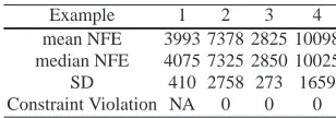
probability factor,η used in SR was set to 0.45. Table 7 reports the mean,median and standard deviations (SD) of the number of function evaluations (NFE) over the 30 independent runs of DEBLP-SR to meet the convergence criteria (i.e. UPO attains the value of at least 1×10−8_).

Table 7 Summary of Performance of DEBLP-SR on GNEP Examples

Example 1 2 3 4 mean NFE 3993 7378 2825 10098 median NFE 4075 7325 2850 10025 SD 410 2758 273 1659 Constraint Violation NA 0 0 0

While it is clear that all the examples are easily solved using DEBLP-SR, three observations are pertinent from Table 7. Firstly, comparing Problem 3 and 4 for example, we can see that as the dimensions increase, the NFE required to meet the convergence criteria also increase significantly. This is a manifestation of the so called “curse of dimensionality” [10] which plagues optimisation algorithms in general and meta-heuristics in particular. Secondly the mean and median NFE re-quired to solve the GNEP (Example 2) is almost twice that rere-quired to solve the NEP (Example 1). This should not come as a surprise because constrained problems are known [121] to be harder to solve than unconstrained ones. Finally, the constraint violation of all examples at termination is 0 as shown in the last row of Table 7. Thus we can conclude that the SR method for handling constraints is effective for the examples given.

8 Summary and Conclusions

8.1 Summary

In this chapter, we have outlined a meta-heuristic algorithm DEBLP to solve bi-level programming problems. These hierarchical optimisation problems are typi-cally characterised by non convexity and non smoothness. DEBLP is designed to synergise the well-documented global search capability of Differential Evolution with the application of robust deterministic optimisation techniques to the lower level problem. Most importantly, DEBLP is fully consistent with the Stackleberg framework upon which the BLPP is founded where the leader takes into account the follower’s decision variables when optimizing his objective and where the follower treats the leader’s variables as exogenous when solving his problem.

was the regulatory agency and the followers were users of the highway network. The BLPPs from this field were shown to be MPECs as the lower level problem arises naturally as a Variational Inequality. We also examined examples from Pa-rameter Estimation Problems, a key step in the development of models in science and engineering applications, which could also be formulated as BLPPs. In order to enable DEBLP to solve BLPPs where the upper level problem was also subject to general constraints, we integrated the stochastic ranking algorithm from [99] into DEBLP to produce DEBLP-SR. Stochastic ranking is a constraint handling tech-nique that seeks to balance the dominance of the objective and constraint violations in the search process of meta-heuristic algorithms. We demonstrated the operation of DEBLP-SR on a series of Generalised Nash Equilibrium Problems which could be formulated as BLPPs characterised by upper level constraints. Developments in the literature of GNEPs also enabled us to even specify a specific termination crite-ria for the proposed BLPP and hence provides additional justification for the use of a meta-heuristic for these problems.

Due to space constraints, we could not illustrate BLPPs where the leader’s deci-sion variables and/or the follower’s variables were restricted to be discrete or binary. However there exists a large body of literature of DE being used for such problems, albeit single level ones [91, 92]. Thus we conjecture the techniques proposed therein could be integrated into DEBLP to solve such problems as well. Additionally dis-crete and mixed integer lower level problems can already be solved using established techniques available in the deterministic optimisation literature [9, 70, 85].

8.2 Further Research

In this chapter, we have demonstrated that DEBLP is an effective meta-heuristic for a variety of BLPPs. Nevertheless there are several topics that still require additional research before robust methodologies can be developed. The study of some of these problems is still in its infancy but we argue that meta-heuristic paradigms such as Differential Evolution can provide a viable alternative solution framework for these.

8.2.1 Multiple Optimisation Problems at Lower Level

8.2.2 Bi-Level Multiobjective Problems

Recall that in our formulation of the BLPP in Eq. 1 we assumed the function map-pings: U,L :Rn1_×Rn2 _→R1_{. In other words, the objectives in both the upper and}

lower levels are restricted to be scalar. However there are also problems where the objectives are vectors. Such problems are known as multiobjective (MO) prob-lems i.e. where the decision maker has multiple, usually conflicting, objectives. In such problems the Pareto Optimality criteria is used to identify optimum solutions [30, 90]. One of the major advantages of using population based meta-heuristic al-gorithms for MO Problems is that because of their population based structure, they are able to identify multiple Pareto Optimal solutions in a single run [29].

Two categories of these problems have been discussed in the literature. Firstly there is the case where only the upper level objective is vector based or secondly where both the upper and lower level objectives are vector based. For problems occurring in the first category, advances in meta-heuristics to solve MO problems (e.g. [30]) could be easily integrated into DEBLP to transform it into an algorithm able of handle MO-BLPPs of the type described in e.g. [44, 110, 123]. Problems of the second category are relatively novel in the literature and have only recently been investigated [31]. Further research should introduce new methodologies to enable DEBLP to solve problems in this latter category.

8.2.3 Multiple Leader Follower Games

In Section 4 we provided an example of the COTP which models a highway reg-ulatory agency optimising the total travel time on the highway system by levying toll charges. With the trend in recent years towards privatization together with con-strained governmental budgets, it is quite possible that instead of a welfare maxi-mizing authority setting the tolls in future, this task could potentially be consigned to private profit maximising entities. The latter obtain concessions to collect tolls from users on these private toll roads [36, 119] in return for providing the capital layout of investments in new road infrastructure. When setting such tolls, these pri-vate firms could also be in competition with others doing the same on other roads in the network.

The problem just described is in fact an example of a class of Equilibrium prob-lems with Equilibrium Constraints (EPEC). In EPECs, the decision variables of the private firms are constrained by a variational inequality describing equilibrium in some parametric system [62]. For example in the case of competition between the private toll road operators just highlighted, the equilibrium constraint is just Wardrop’s User Equilibrium condition. The study of EPECs has recently been given greater emphasis by researchers in many disciplines [55, 68, 77, 80, 119, 125]. Though it is still in a period of infancy it has emerged as major area of research [22, 35, 109] in applied mathematics.

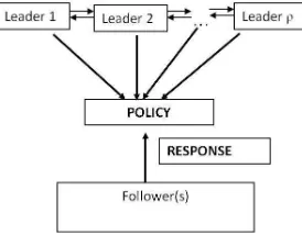
de-cision variables of other MPECs [125]. Compared to the MPEC, the focus in the EPEC is shifted away from finding minimum points to finding equilibrium points [78, 79]. Figure 4 gives a multi-leader generalization of the BLPP that constitutes a Multi-leader-follower game [68] where there are nowρ,ρ>1 leaders instead.

In this multi-leader generalization of the Stackelberg game researchers have con-jectured that there could be two possible behaviours of the leaders at the upper level [78, 88]. At one end, leaders could cooperate which results in a multiobjective prob-lem subject to an equilibrium constraint at the lower level [120]. At the other end, the leaders could act non-cooperatively and play a Nash game amongst themselves resulting in a Non Cooperative EPEC (NCEPEC). EPECs are extremely difficult to solve and the current emphasis has been on the use of nonsmooth methods and nondifferentiable optimisation techniques [78, 79]. We believe that meta-heuristic algorithms offer a powerful alternative solution methodology for EPECs in both cases. In the case when leaders are assumed to cooperate, we have pointed out that because they operate with populations, population based meta-heuristics are able to identify multiple Pareto Optimal solutions in a single simulation run. This is key to solving multiobjective problems. For the NCEPECs, a DE based algorithm ex-ploiting a concept from [71] was proposed and demonstrated on a range of EPECs occurring in transportation and electricity markets in [62].

Most importantly, whatever solution algorithms are proposed in future, when searching for an equilibrium amongst the players at the upper level they must con-tinue to take the reaction of the followers at the lower level into account. This serves to ensure that proposals are entirely consistent with the Stackleberg paradigm which remains applicable in EPECs.

Fig. 4 Pictoral Representation of an EPEC

Acknowledgements The research reported here is funded by the Engineering and Physical