Local binary regression with spherical predictors

This is a repository copy of Local binary regression with spherical predictors.

White Rose Research Online URL for this paper:

http://eprints.whiterose.ac.uk/138926/

Version: Accepted Version

Article:

Di Marzio, M, Fensore, S, Panzera, A et al. (1 more author) (2019) Local binary regression

with spherical predictors. Statistics and Probability Letters, 144. pp. 30-36. ISSN

0167-7152

https://doi.org/10.1016/j.spl.2018.07.019

© 2018 Elsevier B.V. This manuscript version is made available under the CC-BY-NC-ND

4.0 license http://creativecommons.org/licenses/by-nc-nd/4.0/.

Reuse

This article is distributed under the terms of the Creative Commons Attribution-NonCommercial-NoDerivs (CC BY-NC-ND) licence. This licence only allows you to download this work and share it with others as long as you credit the authors, but you can’t change the article in any way or use it commercially. More

information and the full terms of the licence here: https://creativecommons.org/licenses/

Takedown

If you consider content in White Rose Research Online to be in breach of UK law, please notify us by

Local binary regression with spherical predictors

Marco Di Marzioa,∗, Stefania Fensorea, Agnese Panzerab, Charles C. Taylorc

a_{DSFPEQ, Universit´a di Chieti-Pescara, viale Pindaro 42, 65127 Pescara, Italy}

b_{DiSIA, Universit´a di Firenze, viale Morgagni 59, 50134 Florence, Italy}

c_{Department of Statistics, University of Leeds, Leeds LS2 9JT, UK}

Abstract

We discuss some classes of local estimators for regression when the predictor lies

on the d-dimensional sphere and a binary response. In particular, we adapt the theory of

local polynomial regression and local likelihood estimation to deal with the problem at

hand. We provide asymptotic L2properties for some estimators in these classes along

with some simulations and a real-data application.

Keywords: Directional data, Local likelihood, Local polynomials, Spherical kernels,

Tangent-normal decomposition

MSC:

1. Introduction

Data lying on the unit hypersphere embedded inR

d_{, d≥2, arise in many scientific}

fields. They are typically referred as directional or spherical data. Classical examples,

when d=2, are directions of winds and marine currents, and directions of flight of

birds from a point of release. Also, locations on the surface of the ordinary sphere

(d=3) are ubiquitous in Earth and planetary sciences. Fields of recent interest for

directional data include genome sequence representations, text analysis and clustering,

morphometrics, and computer vision, see, for example, Hamsici and Martinez (2007).

∗_{Corresponding author}

Email addresses:[email protected](Marco Di Marzio),[email protected]

The non-linear nature of the hypersphere sets apart directional statistics from

stan-dard methods, which are typically designed for linear data. However, in the last few

decades directional statistics has greatly evolved, and now directional counterparts of

many classical statistical methods exist. Classical comprehensive accounts of

direc-tional statistics are provided by Batschelet (1981), Fisher et al. (1987), and Mardia and

Jupp (2008), and more recently by Ley and Verdebout (2017, 2018).

Kernel-based methods for regression estimation when the response is a linear

vari-able and the predictor has a directional nature have been recently studied. Indeed,

the absence of a boundary on a spherical domain makes smoothing methods – which

typically suffer from boundary bias – well-suited for analysing directional data. In

particular, the local polynomial regression for linear response has been studied by Di

Marzio et al. (2009) in the case of circular predictors, and by Di Marzio et al. (2014)

in the case of a general d-dimensional spherical predictor, as an intermediate step in

the spherical-spherical regression estimation. Then, this topic has been also studied by

Garc´ıa-Portugu´es et al. (2016) in the context of goodness-of-fit tests.

Conversely, the special case of a binary response and a directional predictor by

means of nonparametric regression methods seems to be unexplored, while for a

para-metric approach see Fernandes and Cardoso (2016) and references therein. The binary

regression problem, apart from being of interest per se, is also useful for classification

purposes. Nonparametric methods for classification of directional data, based on kernel

estimation of spherical densities, have been studied by Di Marzio et al. (2018b).

In the Euclidean setting, kernel-based estimators of the binary regression with a

linear predictor have been studied by Fan et al. (1995) and Signorini and Jones (2004),

who provided asymptotic properties of various versions of the estimators. The

dis-cussed methods essentially rely on local polynomial regression and a local likelihood

approach. In this paper we discuss both local polynomial and local likelihood

local-likelihood-based approach has been also investigated in Di Marzio et al. (2017) in the different

context of estimation of densities defined on the d-dimensional torus.

The paper is organized as follows. In Section 2 we recall a Taylor-like polynomial

to approximate functions having the unit hypersphere as their domain. In Section 3 we

discuss the adaptation of the theory of local polynomial regression with a directional

predictor to the binary response case, while, in Section 4 we propose the nonparametric

estimation using a locally weighted likelihood objective function. Finally, Section 5

collects some simulation examples and a real-data application.

2. Series expansion for functions on the sphere

LetS

d−1_={xxx∈

R

d_{:||xxx||=1}denote the unit hypersphere embedded in}

R

d_{, d≥2.}

The tangent-normal decomposition provides a possible parametrization of a point on

S

d−1_{. Specifically, for fixed xxx∈}

S

d−1_{, according to the tangent-normal decomposition,}

any vector uuu∈S

d−1_{can be expressed as}

u u

u(ξξξ,θ) =xxx cos(θ) +ξξξsin(θ),

whereθ is the angle between uuu and xxx, andξξξ is a unit vector orthogonal to xxx. Now,

lettingµ_ddenote the Lebesgue measure ofS

d_{, with}

ωd=µd

S

d₌ 2π(d+1)/2

Γ((d+1)/2),

and settingTxxx={ξξξ∈S

d−1_{:ξξξ ⊥xxx}, for a real-valued function g defined on}

S

d−1_{, the}

integration formula corresponding to the above parametrization is

Z

S

d−1g(uuu)dµd−1(uuu) =

Z π

0

sind−2(θ)dθ

Z

Txxx

g(uuu(ξξξ,θ))dµd−2(ξξξ). (1)

Moreover, letting ¯g(xxx):=g(xxx/||xxx||)be the homogeneous extension of g to R

{000d}, with 000dbeing the d-dimensional zero vector, we have that

∂ℓ

∂θℓg(uuu(ξξξ,θ))

_θ=0

=D(ℓ) ξξξ g(xxx)¯ ,

whereD(ℓ)

ξξξ g(xxx)¯ is the directional derivative of orderℓof ¯g at xxx in the direction ofξξξ. ClearlyD(0)

ξξξ g(xxx) =¯ g(xxx), while, letting∇ℓg¯(xxx)be the matrix of the derivatives of total

orderℓof ¯g at xxx, one has

D(ℓ)

ξξξ g(xxx) =¯ ξξξ′∇ℓg¯(xxx)ξξξ ⊗(ℓ−1)

,

where aaa⊗ℓ stands for the Kroneckerian power of order ℓ of a vector aaa. Then, for

example, we haveD(1)

ξξξ g(xxx) =¯ ξξξ′∇g¯(xxx)and D_ξξξ(2)g(xxx) =¯ ξξξ′∇2g¯(xxx)ξξξ, with ∇1g¯(xxx) and ∇2

¯

g(xxx)respectively being the gradient vector and the Hessian matrix of ¯g at xxx, while

D(3)

ξξξ g(xxx) =¯ ξξξ′∇3g¯(xxx)ξξξ⊗ξξξ, with aaa⊗aaa being the Kroneckerian product of the vector aaa

by itself.

Now, under suitable continuity assumptions, a Taylor-like expansion of a real

val-ued function g defined onS

d−1_{can be provided. Specifically, by assuming the}

conti-nuity of∇ℓ_g¯(xxx), xxx∈S

d−1_{, forℓ∈(1, . . . ,p), a pth-order series expansion of g around xxx}

yields

g(uuu)≈g(xxx) +

p

∑

ℓ=1

θℓ

ℓ!D

(ℓ)

ξξξ g(xxx)¯

=g(xxx) +

p

∑

ℓ=1

θℓ

ℓ!ξξξ ′_∇ℓ

¯

g(xxx)ξξξ

⊗(ℓ−1)

. (2)

The above expansion has been employed for deriving the asymptotic properties of

ker-nel estimators for spherical densities by Hall et al. (1987) and Klemela (2000), to obtain

a component-wise local approximation of spherical-spherical regression by Di Marzio

et al. (2014), and to approximate the entries of skew-symmetric matrices and define

3. Local polynomial binary regression

Let(XXX,Y)be aS

d−1_{× {0,1}-valued random variable, and set}λ_{(xxx) =P(Y =1|}

X X

X=xxx). If independent copies(XXX1,Y1), . . . ,(XXXn,Yn)of(XXX,Y)are observed, by

ignor-ing the binary nature of YYY , a naive nonparametric estimation ofλ(xxx)can be performed

by using the local polynomial estimators with real-valued response and spherical

pre-dictor, which have been studied by Di Marzio et al. (2014).

In particular, following this approach, the regression function at XXXiis approximated

by a suitable pth degree polynomial around xxx∈S

d−1_{, and a local estimator of}λ_(xxx)is

defined as the solution (for the zero order coefficient) of the minimization of a weighted

L2distance between the Yis and the approximating polynomial. Different values of p

give different estimators. Formally, by using expansion (2), a pth degree local

poly-nomial estimator ofλ at xxx∈S

d−1_{, say ˆλ(xxx; p), can be defined as the solution forβ} 0

of

argmin

{β0,βββ1,...,βββp}

n

∑

i=1

(

Yi−β0−

p

∑

ℓ=1

θℓ i

ℓ ξξξ

′

iβββℓξξξ

⊗(ℓ−1)

i

)2

K_κ(xxx′XXXi), (3)

whereθi is the angle between XXXi and xxx, and the weight Kκ is a spherical kernel. A

spherical kernel can be essentially defined as a unimodal density havingS

d−1 _{as its}

support, with rotational symmetry about its mean directionµµµ= (0, . . . ,0,1), and

con-centration parameterκ >0 such that asκ increases K_κ concentrates aroundµµµ. In

equation (3) the weight function emphasizes the contribution of the observations XXXis

which are closer to the estimation point xxx. Kernels of this form have been used by Hall

et al. (1987) for density estimation on the sphere and by Di Marzio et al. (2014) and Di

Marzio et al. (2018a) for spherical-spherical regression estimation.

Now, when p=0, the solution forβ0leads to the local constant estimator

ˆ

λ(xxx; 0) =∑

n

i=1YiKκ(xxx′XXXi)

∑n

i=1Kκ(xxx′XXXi)

, (4)

a suitable constraint (see Di Marzio et al. (2014) for details) can be expressed as

ˆ

λ(xxx; 1) =

n

∑

i=1

W_κ(xxx′XXXi)Yi,

where

W_κ(xxx′XXXi) =xxx′

(

n

∑

j=1

K_κ(xxx′XXXj)(xxx+θjξξξj)(xxx+θjξξξj)′

)−1

(xxx+θiξξξi)Kκ(xxx′XXXi).

Now, in order to discuss the asymptotic properties of the estimators, we need to

recall the spherical counterparts of the jth moment, j∈N, and the roughness of a

Euclidean kernel, which, for a kernel K_κ, respectively are

bj(κ) =ωd−2

Z π

0

K_κ(cos(θ))θjsind−2(θ)dθ,

and

ν0(κ) =ωd−2

Z π

0

K_κ2(cos(θ))sind−2(θ)dθ.

Let Tr(AAA)denote the trace of the matrix AAA, and use f to denote the common density

of the XXXis. Then, for the cases p=0 and p=1, by respectively using results in Theorem

1 and Theorem 2 in Di Marzio et al. (2014), we obtain the following

Result 1. Given theS

d−1_{× {0,1}-valued random sample(XXX}

1,Y1), . . . ,(XXXn,Yn),

con-sider estimator ˆλ(xxx; p), xxx∈S

d−1_{. If}

i) K_κ is a spherical kernel such that as n increases b2(κ)andν0(κ)/n both go to 0, and for j>2, bj(Kκ) =o(b2(κ));

ii) f(xxx)>0 and all the entries of∇_f¯(xxx),∇_λ¯(xxx), and∇2_λ¯(xxx)are continuous,

then

E_[λˆ_{(xxx; 0)]−}λ_{(xxx) =} b2(κ)

2(d−1) Tr n

∇2 ¯ λ(xxx)

o

+2∇

′

¯

λ(xxx)∇_f¯(xxx)

f(xxx) !

+o(b2(κ)),

E_[λˆ_{(xxx; 1)]−}λ_{(xxx) =} b2(κ)

2(d−1)Tr n

∇2 ¯ λ(xxx)

o

and, for both p=0 and p=1,

Var_[λˆ_{(xxx; p)] =}ν0(κ)

n

λ(xxx)(1−λ(xxx))

f(xxx) +o

ν

0(κ)

n

.

Remark 1. Recently, Garc´ıa-Portugu´es et al. (2016) proposed a different series

ex-pansion of the regression function with linear response and directional predictor, which generalizes the proposal of Di Marzio et al. (2009) in the circular case when p=1.

The optimization of the corresponding L2loss leads to a projected local linear

estima-tor which shares the asymptotic properties of the local linear estimaestima-tor of Di Marzio et al. (2014).

An optimal smoothing degree would minimize the asymptotic mean-squared error

of ˆλ(xxx; p), which is the sum of the leading terms of the asymptotic squared bias and the

asymptotic variance. Notice that the dependence of asymptotic bias and variance on

the concentration parameter cannot be generalized with respect to the kernel, because

it is not a scale factor.

For the important case of a von Mises-Fisher kernel (which can be regarded as the

spherical counterpart of the Gaussian kernel), and is defined onS

d−1_as

K_κ(xxx′µµµ) = κ

d/2−1

(2π)d/2_I

d/2−1(κ)

exp(κxxx′µµµ),

withI_{u(·)being the modified Bessel function of the first kind and order u, when}κ_is

big enough, and j∈N, the following approximations of bj(κ)andν0(κ)hold

bj(κ)∼

2j/2Γ((d+j−1)/2)

κj/2Γ_((d−1)/2) , and ν0(κ)∼

κ(d−1)/2

2d−1π(d−1)/2. (5)

As a consequence, when K_κ is a von Mises-Fisher kernel, the asymptotic bias and the

asymptotic variance, for both p=0 and p=1, are

E_[λˆ_{(xxx; p)]−}λ_{(xxx) =}O

₁

κ

, and Var_[λˆ_{(xxx; p)] =}O κ

(d−1)/2

n !

.

Then, in the case of a von Mises-Fisher kernel, for both local constant and local

O(n2/(d+3)_{)and gives a convergence rate of magnitude O(n}−4/(d+3)_{). This is the same}

rate attained by single bandwidth local constant and local linear estimators of a

real-valued regression function defined onR

d−1_{, when a second-order kernel is employed.}

4. Local logistic regression via likelihood

The approach discussed in the previous section does not produce bona-fide

esti-mates when the polynomial degree is greater than 0. Despite the fact that a truncation

could be used for exploratory data analysis, the subsequent lack of differentiability may

be a serious issue. To take into account the binary nature of the response, one should

consider the estimator as the optimiser of a more suited objective function, such as the

log-likelihood one, instead of the least squares in(3).

Specifically, given theS

d−1_{× {0,1}-valued random sample(XXX}

1,Y1), . . . ,(XXXn,Yn),

the log-likelihood connected with the binary regression is

n

∑

i=1

{Yilog(λ(XXXi)) + (1−Yi)log(1−λ(XXXi))}.

The locally weighted version, at xxx∈S

d−1_{, of the above log-likelihood can be}

ex-pressed as

n

∑

i=1

Yilog

λ_(XXX

i)

1−λ(XXXi)

+log(1−λ(XXXi))

K_κ(xxx′XXXi),

where K_κ(xxx′XXXi)is a spherical kernel with mean direction XXXi, and evaluated at xxx. Setting

δ=log(λ/(1−λ)), the above expression can be re-written as

n

∑

i=1

{Yiδ(XXXi)−log(1+exp(δ(XXXi)))}Kκ(xxx′XXXi),

and, approximatingδ(XXXi)around xxx in the local log-likelihood function by using

ex-pansion (2), a class of nonparametric estimators forλ(xxx)can be obtained. Specifically,

of ¯δ at xxx. Then, for fixed xxx∈S

d−1_{, by expressing XXX}

iaccording to the tangent normal

decomposition, we define

qp(XXXi;β0,βββ1, . . . ,βββp) =β0+

p

∑

ℓ=1

θℓ i

ℓ!ξξξ ′

iβββℓξξξ⊗(ℓ−

1)

i .

Hence, under suitable smoothness assumptions, the p-degree expansion of the

log-likelihood can be expressed as

n

∑

i=1

Yiqp(XXXi;β0,βββ1, . . . ,βββp)−log(1+exp(qp(XXXi;β0,βββ1, . . . ,βββp))) Kκ(XXX′ixxx). (6)

It is interesting to note that, whenκ goes to 0, the kernel K_κ(xxx′XXXi)approaches

the uniform density and assigns the same weight to each sample point, for any xxx. As

a consequence, forκ going to 0, the local log-likelihood optimization reduces to the

standard logistic regression problem with spherical predictor.

Now, letting ˆβ0be the solution forβ0of the maximization of (6) with respect to

{β0,βββ1, . . . ,βββp}, a p-degree local polynomial estimator forλ(xxx)is

ˆ

λL(xxx; p) =

exp(βˆ0)

1+exp(βˆ0)

.

When p=0, the resulting estimator is the local constant one previously discussed,

while, when p=1, we obtain the spherical version of the local linear logistic estimator

studied in the Euclidean setting by Fan et al. (1995) and Signorini and Jones (2004).

A closed-form expression for ˆλL(xxx; 1)does not exist, but, obviously, distinctly from

ˆ

λ(xxx; 1), the estimator always takes value on[0,1].

Concerning the asymptotic properties, by reasoning as in Theorem 3 and Theorem

4 of Fan et al. (1995) with g being the logit link, and by using Result 1, we get the

following

Result 2. Given a S

d−1_{× {0,1}-valued random sample (XXX}

1,Y1), . . . ,(XXXn,Yn),

con-sider the estimator ˆλL(xxx; 1), xxx∈S

hold, then

E_[λˆ_{L(xxx; 1)]−}λ_{(xxx) =} b2(κ)

2(d−1)Tr n

∇2 ¯ δ(xxx)

o

λ(xxx)(1−λ(xxx)) +o(b2(κ)),

and

Var_[λˆ_{L(xxx; 1)] =}ν0(κ)

n

λ(xxx)(1−λ(xxx))

f(xxx) +o

ν

0(κ)

n

.

Notice that ˆλL(xxx; 1)shares both the asymptotic variance and the order of the

asymp-totic bias of ˆλ(xxx; p), p∈(0,1). Moreover, the asymptotic bias depends only onλ and

the derivatives of ¯λ but not on f , as it happens for ˆλ(xxx; 1).

Clearly, by virtue of Result 2, if a von Mises-Fisher kernel is employed as the

weight, by recalling the approximations in (3), the estimator attains the convergence

rate of order n−4/(d+3)_.

Concerning the selection ofκ, a possible way is to start from a least-squares

objec-tive function, and choose the value ofκwhich minimizes

n

∑

i=1

Yi−λˆ−i(XXXi;κ)

2

,

where ˆλ−i(XXXi;κ)stands for the estimate of λ at XXXi with the ith sample observation

removed. A more natural way is to start from the leave-one-out version of the local

log-likelihood, i.e. to select the value ofκmaximizing

n

∑

i=1

(

Yilog

ˆ

λ−i(XXXi;κ)

1−λˆ−i(XXXi;κ)

!

+log1−λˆ−i(XXXi;κ)

)

. (7)

Remark 2. A possible generalization of the discussed approach arises from

consider-ing different weights for successes and failures in the local log-likelihood expression, i.e.

n

∑

i=1

Yiqp XXXi;β0,βββ1, . . . ,βββp

K_κ1(xxx′XXXi)−log 1+exp(qp(XXXi;β0,βββ1, . . . ,βββp))

K_κ2(xxx′XXXi),

with K_κ1 and K_κ2 being spherical kernels giving weight to the observations of the pre-dictor corresponding to Y=1 and Y=0, respectively.

When p=0, the solution forβ0of the maximization of the above local log-likelihood

is defined by using the kernel estimators, say ˆf1(xxx;κ1)and ˆf2(xxx;κ2), of the spherical

densities f1and f2respectively characterizing the distributions of the predictor in the

spaces of successes and failures, based on random samples of respective sizes n1and

n2, i.e.

ˆ

λ(xxx;κ1,κ2) =

n1fˆ1(xxx;κ1)

n1fˆ1(xxx;κ1) +n2fˆ2(xxx;κ2)

. (8)

5. Numerical examples

5.1. Simulation

In this section we use simulation experiments to test the performance of the

pro-posed estimator for classification tasks. In particular, we consider the problem of

as-signing label 0 or 1 to an observation xxx∈S

d−1_{. To this end, we adopt the rule according}

to which xxx is assigned to the population with label 1 if the estimate ofλ(xxx)is greater

or equal to 0.5.

We use vMF(µµµ,γ)to denote the von Mises-Fisher distribution onS

2_{with mean}

directionµµµ (polar co-ordinates expressed in degrees) and concentration parameterγ.

We consider different experiments using the following scenarios, where samples of

sizes n1=n2=200 are respectively drawn from vMF(µµµ1,γ1)and vMF(µµµ2,γ2):

Scenario 1:µµµ₁= (270,20),µµµ₂= (270,−20)andγ1=γ2=10;

Scenario 2:µµµ₁= (270,20),µµµ₂= (270,−20)andγ1=γ2=20;

Scenario 3:µµµ₁= (270,20),µµµ₂= (220,−20),γ1=5 andγ2=10.

In Scenario 1 the populations, which share the longitude of the mean direction and

the value of the concentration parameter, generate rather overlapping groups. Scenario

2 refers to more concentrated populations generating more separated groups. Finally,

in Scenario 3 two well-separated groups are generated by populations with different

co-ordinates of the mean directions and different concentrations.

In the first experiment we consider the estimator (8) with K_κ1 and K_κ2 both being

von Fisher kernels. The smoothing degrees are selected using the von

-90 135 90 45 180 225 X O X O O X X O X OX O X XO X O O X XO O X O X O X O

XXOXO

X O X O O X XXX XO

O

X

270XO

XO O X XO X O X O O X X O

XOX O X O X O O X O O X O X X O X O X O O O X X XO O XX O X O X O X O XO O O

X XOXO

XO

XO XO

XO O X O O X XO 45 90 X O -45 315 O X O X 0 0 -90 135 90 45 180 225 O X

OOX X XXX

O

X

O

XXO

XO O X 270O O X O X XO X O X O O X X X X O X XX X X X O OX O X X X O X O X X X X X O X X X X X O

XO_XXX X X

45 90 -45 315 0 0 -90

135 90 45

XX O X OO O X225 180 X O O X X O O X O X O X X O O X O O O X X X O X X X O OO O OX O X X O XO O OXO

O X O X O X O X X O O X X O XO X O XX O X 270 -45 315 0 0 45 90

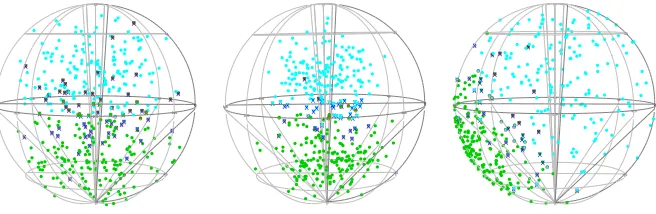
Figure 1: From left: Misclassified observations using KDE classification (marked by ‘X’) and using lo-cal likelihood with p=0 (marked by ‘o’) for one dataset drawn from vMF(µµµ111,γ1)(cyan points) and

vMF(µµµ222,γ2)(green points) in scenarios 1, 2 and 3.

we consider estimator (4). Also in this case we use the von Mises-Fisher kernel as

the weight, by selecting the concentration parameter by least squares cross-validation.

Figure 1 illustrates the misclassified observations obtained according to the rule for

estimators (8) and (4) by using one dataset for each of the described scenarios. In

Table 1, for each experiment, we report as the accuracy measure the average

misclas-sification rate over 200 simulated datasets. The results show that the binary regression

estimator slightly outperforms the kernel density classifier (KDE), especially when the

groups are well-separated. Moreover, the results for n1=n2show that, in the

con-sidered scenarios, estimator (4) performs slightly better than the same estimator using

two concentration parameters (which leads to the same classification rule as the kernel

density one).

Table 1: Estimate of the misclassification rates for kernel density classification and local binary regression with p=0, using 200 samples of sizes n1=n2=200 respectively drawn from fj=vMF(µµµj,γj),j∈(1,2),

given in scenarios 1–3. For both classification rules we use a von Mises-Fisher kernel: for KDE,κ1andκ2 are selected according to the von Mises-Fisher reference rule, and for the local binary regression estimatorκ is selected by least squares cross validation.

Classification rule Misclassification rate

Scenario 1 Scenario 2 Scenario 3

KDE estimator 0.178 0.090 0.112

5.2. Handwritten digit recognition

We apply our methods to the digits dataset used in the StatLog project (Michie

et al., 1994). The dataset consists of 18,000 examples of the digits 0 to 9 (i.e. q=

10 classes) extracted from hand-written postcodes in Germany. These numbers were

initially digitised onto 16×16 images with 256 grey levels; examples are shown in

Figure 2. To enable meaningful comparisons with previously obtained results, we have

used the same train-test split of the data which has 900 examples of each number (0–9)

in the training set and the test set, and an averaging over 4×4 pixels resulting in 16

real-valued variables. These data were then transformed to the unit sphere by simply

normalizing each observation replacing XXXiby XXXi/||XXXi||.

Figure 2: Examples of 10 handwritten, digitised digits with resolution 16×16 and 256 grey scales, extracted from postcodes in Germany (Michie et al., 1994).

Our implementation, which corresponds to a 1-degree local polyomial estimator,

used logistic regression with weights obtained from a spherical kernel. The smoothing

parameter was selected — for each pair of classes(j,k)∈ {0,1, . . . ,9} × {0,1, . . .,9}

—using cross-validation (i.e. Equation (7)), which yielded solutions for the smoothing

parameter ranging from 0.9 to 38.8. Then, for each element of the test set, we compute

the probability of membership of class j, given an alternative of class k, say Pjk with

Pjk=1−Pk j(also setting Pj j=1), using the correspondingκjk(=κk j)found by

cross-validation. Finally, we allocate this observation to the class argmax_kminjPjk. The error

rate for 9000 observations in the test set, was 0.043, which is much better than the

unweighted multinomial logistic regression (error 0.086), a simple linear discriminant

(0.114) and just better than the top rank classifier (k-nearest neighbour, with an error

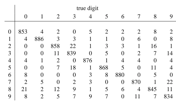
rate of 0.047) of those given in (Michie et al., 1994, p. 136). The confusion matrix

classification mistakes were to recognize an ”8” as a “0”, a “2” as a “3”, and a ”7” as a

”9”.

true digit

0 1 2 3 4 5 6 7 8 9

0 853 4 2 0 5 2 2 2 8 2

1 4 886 3 3 1 1 0 6 0 8

2 0 0 858 22 1 3 3 1 16 1

3 0 0 11 839 0 5 0 2 7 14

4 4 1 2 0 876 1 4 4 0 4

5 0 0 7 18 1 868 5 0 11 4

6 8 0 0 0 3 8 880 0 5 0

7 2 5 0 2 3 0 0 870 1 22

8 21 2 12 9 1 5 6 4 845 11

9 8 2 5 7 9 7 0 11 7 834

Figure 3: Confusion matrix for local multinomial logistic classifier applied to German handwritten postcode digits. Columns represent true label, and rows the predicted label.

Although the error rate is very good, we note that this approach was

computation-ally intensive, with the multinomial logistic model entailing the estimation of q(q−

1)/2=45 smoothing parameters in the training phase, and a further fitting of nq(q−

1)/2=405,000 models in the testing phase. Whilst it would be straightforward to

consider p=2 (including interaction terms, if desired) this would take an excessive

amount of time without a common choice ofκacross all class pairs.

Using a classification rule based on a kernel density estimator, a single

smooth-ing parameter (for all classes) was selected by leave-one-out cross-validation on the

training data. This value ofκ (=140.6) was then used to classify the test data. For

this classifer, the error rate of 0.039 was unexpectedly somewhat better than the result

given in Michie et al. (1994) (0.068) for data which have not been transformed to the

sphere.

References

Di Marzio, M., Fensore, S., Panzera, A., Taylor, C.C., 2017. Circular local likelihood.

TEST 21, 1863–8260.

Di Marzio, M., Fensore, S., Panzera, A., Taylor, C.C., 2018. Kernel density

classifica-tion for spherical data, submitted.

Di Marzio, M., Panzera, A., Taylor, C.C., 2009. Local polynomial regression for

circu-lar predictors. Statistics & Probability Letters 79, 2066–2075.

Di Marzio, M., Panzera, A., Taylor, C.C., 2014. Nonparametric regression for spherical

data. Journal of the American Statistical Association 109, 748–763.

Di Marzio, M., Panzera, A., Taylor, C.C., 2018. Nonparametric rotations for

sphere-sphere regression. Journal of the American Statistical Association, forthcoming.

Fan, J., Heckman, N., Wand, M.P., 1995. Local Polynomial Kernel Regression for

Generalized Linear Models and Quasi-Likelihood Functions. Journal of the

Ameri-can Statistical Association 90, 141–150.

Fernandes, K., Cardoso, J.S., 2016. Discriminative directional classifiers.

Neurocom-puting 207, 141–149.

Fisher, N., Lewis, T., Embleton, B., 1987. Statistical Analysis of Spherical Data.

Cam-bridge University Press.

Garc´ıa-Portugu´es, E., Van Keilegom, I., Crujeiras, R.M., Gonz´alez-Manteiga, W.,

2016. Testing parametric models in linear-directional regression. Scandinavian

Jour-nal of Statistics 43, 1178–1191.

Hall, P., Watson, G., Cabrera, J., 1987. Kernel Density Estimation with Spherical Data.

Biometrika 74, 751–762.

Equivalency of Spherical and Normal Distributions in Classification. The Journal of

Machine Learning Research 8, 1583–1623.

Klemela, J., 2000. Estimation of densities and derivatives of densities with directional

data. Journal of Multivariate Analysis 73, 18–40.

Ley, C., Verdebout, T., 2017. Modern Directional Statistics. Chapman & Hall/CRC

Press, Boca Raton, Florida.

Ley, C., Verdebout, T., 2018. Applied Directional Statistics: Modern Methods and Case

Studies. Chapman & Hall/CRC Press, Boca Raton, Florida.

Mardia, K.V., Jupp, P.E., 2008. Directional Statistics. Chichester: J. Wiley.

Michie, D., Spiegelhalter, D.J. and Taylor, C.C. (eds) 1994. Machine Learning, Neural

and Statistical Classification. Chichester: Ellis Horwood.

Signorini, D.F., Jones, M.C., 2004. Kernel Estimators for Univariate Binary