Development Of Active Steering Control Based On Sliding Mode Control With The Inclusion Of An Observer

(1)

DEVELOPMENT OF ACTIVE STEERING

CONTROL BASED ON SLIDING MODE CONTROL

WITH THE INCLUSION OF AN OBSERVER

NG XUE YAN

(2)

ON SLIDING MODE CONTROL WITH THE INCLUSION OF

AN OBSERVER

NG XUE YAN

This report is submitted in partial fulfilment of the requirements

for the degree of

Bachelor of Electronic Engineering (Industrial Electronics) with

Honours

Faculty of Electronic and Computer Engineering

Universiti Teknikal Malaysia Melaka

(3)

Scanned by CamScanner

UNIVEnSTI TEKNIKAL MALAYSIA MELA KA

C

l!U~~I

FAKULTI KEJURUTERAAN ELEKTRONIK DAN KEJlJRIJ'I ERAAN KOMPUTER

llOltANG l'ENGESAllAN STATUS LAl'OllAN

PRO.JEK SAR.JANA MUDA JI

Tajuk Projck DEVELOPMENT OF ACTIVE STEERING CONTROL BASED ON

SLIDING MODE CONTROL WITH THE INCLUSION OF AN

OBSERVER

Sesi Pengajian 6 I 7

Say a NG XUE YAN

(HURUF BESAR)

mengak."U membenarkan Laporan Projek Sarjana Muda ini disimpan di Perpustakaan dengan syarat-syarat kegunaan seperti berikut:

1. Laporan adalah hakmilik Universiti Teknikal Malaysia Melaka.

2. Perpustakaan dibenarkan membuat salinan untuk tujuan pengajian sahaja.

3. Perpustakaan dibenarkan membuat salinan laporan ini sebagai bahan pertukaran antara institusi

pengajian tinggi.

4. Sila tandakan ( .../ ) :

D

SULIT*

D

TERllAD**

[JJ

TIDAK TERHAD

GAN PENULIS)

. 1(1o/Wt:J.·

Tankh: ... .l ... .

*(Mengandungi maklumat yang berdarjah keselamatan atau kepentingan Malaysia seperti yang termaktub di dalam AKTA RAHSIA RASMI 1972)

.. (Mengandungi maklumat terhad yang telah ditentukan oleh organisasi/badan di mana penyelidikan dijalankan)

.

1/b(?o

f'J--

·

(4)

Scanned by CamScanner

"I declare that this report is the result of my own work except for quotes as cited in the references."

Signature

···f··

·

··

···

·

Author NG XUE YAN

(5)

Scanned by CamScanner

APPROVAL

"I hereby declare that I have read this thesis and in my opinion this thesis is sufficient

in terms of scope and quality for the award of Bachelor of Electronic Engineering

(Industrial Electronic) with Honours."

Signature

Supervisor Name D SADHIQIN BIN MOHD ISIRA

(6)

Special dedication to my beloved parents

Ng Kek Seng and Ong Guat Cheng

Their encouragement and guidance has always be an inspiration to me along this

(7)

i

ABSTRACT

(8)

ABSTRAK

(9)

iii

ACKNOWLEDGEMENTS

I have just completed my Final Year Project (FYP) and report. In the beginning, I

would like to take this opportunity to express my gratefulness to some organization

and individuals who kindly contributed for my final year project in UTeM. With the

cooperation and contributions from all parties, the objectives of the project which are

soft-skills, knowledge and experiences were gained accordingly even this is just part of

the whole project. Furthermore, I would like thank to my supervisor, Dr. Ahmad

Sad-hiqin Bin Mohd Isira for the proper guidance, cooperation and involvement throughout

my Final Year Project. His effort to ensure the successful and comfort ability of

stu-dents under his responsibility was simply not doubtful. Moreover, I would like to

extend my sincere acknowledgement to my parent and family members who have been

very supportive for the past one year. Their understanding and support in term of moral

and financial were entirely significance towards the project completion. Last but not

list, my appreciation goes to my fellow student in UTeM, especially for who are from

FKEKK. Their willingness to help, opinions and suggestions on some matters, advices

and technical knowledge are simply precious while doing upon completion of my final

(10)

LIST OF TABLES

Page

(15)

ix

LIST OF FIGURES

[image:15.595.114.526.102.789.2]

Page

Figure 1.1 Methodology FLow Chart. 5

Figure 2.1 (a) Schematic view of AFS system; (b) 3D-model of planetary

gear set and electric motor [1]. 11

Figure 2.2 Vehicle Axis System after SAE [2]. 12

Figure 2.3 Vehicle Axis System after SAE [2]. 13

Figure 2.4 Two Degree of Freedom Model [2]. 14

Figure 2.5 Three Degree of Freedom Model after Smith [2]. 14

Figure 2.6 Eight Degree of Freedom Model after Smith [2]. 15

Figure 2.7 Unknown rear and front axle lateral forces act on the car body

with mass m and moment of inertia J [3]. 15

Figure 2.8 The steering angleδF =δS+δCis composed of the command

δS, from the driver and the feedback controlled additional angle

δC. 17

Figure 2.9 Single Track Model for Car Steering. 17

Figure 2.10 Lateral forcesFytF at the front wheel in tire coordinates andFyF

in chassis coordinates. 18

Figure 2.11 The path following task. 26

Figure 2.12 The disturbance attenuation task. 26

Figure 2.13 Structure of an observer-based, or model-based controller,

whereLdenotes the observer gain andF the state feedback gain. 31

Figure 3.1 Methodology FLow Chart. 39

Figure 3.2 Block Diagram of the Active Steering Control. 40

Figure 4.1 Crosswind disturbance profile. 56

Figure 4.2 µ-split braking torque disturbance profile. 57

(16)

Figure 4.4 Comparison between all controller with Braking torque

disurbance. 60

Figure 4.5 Comparison between SMC controller and uncontrolled system

with crosswind disurbance. 62

with crosswind disurbance. 63

Figure 4.7 Comparison between SMC controller and Pole Placement

Controller system with crosswind disurbance. 64

Controller system with crosswind disurbance. 65

Figure 4.9 Comparison between SMC controller and LQR Controller

system with crosswind disurbance. 66

system with crosswind disurbance. 67

Figure 4.11 Comparison between SMC controller and Sliding Mode

Observer system with crosswind disurbance. 68

Observer system with crosswind disurbance. 69

Figure 4.13 Comparison between SMC controller, Sliding Mode Observer,

LQR controller and LQR observer system with crosswind

disurbance. 70

LQR controller and LQR observer system with crosswind

disurbance. 71

with braking torque disurbance. 73

with braking torque disurbance. 74

Controller system with braking torque disurbance. 75

Controller system with braking torque disurbance. 76

(17)

xi

system with braking torque disurbance. 78

Observer system with braking torque disurbance. 79

Observer system with braking torque disurbance. 80

LQR controller and LQR observer system with braking torque

disurbance. 81

LQR controller and LQR observer system with braking torque

disurbance. 82

Figure A.1 The Uncontrolled System. 93

Figure A.2 The Pole Placement Controller System. 93

Figure A.3 The LQR Controller System. 94

Figure A.4 The LQR Observer System. 94

Figure A.5 The SMC Controller System. 95

(18)

CHAPTER 1

INTRODUCTION

1.1 Introduction

Nowadays, there is a common problem that will cause the road accident is losing

con-trol of a car at high speeds. Due to the driver’s failure to understand the many road

conditions and situations that could cause the road accidents are being happened in

term of loss of control. A small city car is not designed to be driven at highway speeds

at the same time that the car’s tires with poor grip will increase the chances of losing

control. A new driver or in young age and inexperience driver will not able to fully

control the car during there are the hidden dangers of disturbances.

Besides that, a well maintained vehicle will also have chances to lose control

due to external factors. There are many external disturbance that may cause a car to

lose control such as crosswind, braking torque rainy day, conditions of the road and

others. Although there are many controllers such as antilock brake system, traction

control, dynamic stability control and active steering are being installed on a vehicle,

these system is still unable to defy extreme forces. Thus, the active steering control is

developed in order to improve the drivability of a vehicle when there are any

distur-bances such as poor road adhesion and crosswinds.

Recently, there are a lot of the researches from all over the world are doing

research about the area of vehicle stability in sequence to the increasing of vehicle

capabilities. This includes the steering control by using different controller strategies

to improve safety and handling for the car steering in order to make sure that the

driver and the passenger are safe. There are a lot of analysis about the steering and

the controller strategy of the dynamic system. However, it is still difficult to value the

(19)

2

A complementary system for a front-steered vehicle that adds or subtracts a

component to the steering signal which is performed by the driver is known as a

steer-ing control system. An angular movement on the steersteer-ing wheel is the steersteer-ing signal

from the driver. The resulting steering angle is thus composed by the component

per-formed by the driver and the component contributed by the steering system. Thus, the

input of the system came from the front wheel angle of the driver. There are many types

of control strategy can be used to stabilize the vehicle during disturbances happened

whether using conventional controller such as PID, fuzzy logic control and sliding

mode control. In this project, a single track car mathematical model and Sliding Mode

Control are implemented and analyzed. The main aimed of this project is to implement

a steering aid system to help the driver.

1.2 Project Overview

There are already exist the driver assistant systems which use a braking method that

been applied on each wheel [4]. Due to the hardware that is consisting the exist of ABS

braking system with an additional yaw rate sensor and does not require a new actuator,

thus these systems are cheap.

There are several reasons that the causes of an active steering system is

consid-ered as a good alternative. The first reason is a torque which is tire force times lever

arm is generated to compensate yaw disturbance torques. The second reason is the

cause of the disturbance torque is the different friction coefficient, µ on the left and

right sides (µ-split braking). On the other side, the braking torque can be

compen-sated and a straight short braking path can be achieved by a steering torque. While the

third reason of an active steering should be a good alternative is energy conservation,

reduced wear of tires and brakes and smooth operation around zero correction.

Practically, braking systems are not capable of immediately react to an

emer-gency situation and cannot immediately compensate small errors. However, it will late

react in detected emergency situations when the car is close to skidding or rolling. The

active steering system is the only feasible way for continuous operation and also for

(20)

Due to modeling inaccuracies, the vehicle dynamics are subjected to various

uncertainties [5]. Thus, this situation is not capable to be handled by the conventional

linear control. Hence, by applying a robust controller to the vehicle system design, the

robust performance capabilities against uncertainties can be overcome.

The main aim of this project is to revise and define the automatic steering

con-trol of passenger cars for general lane-following maneuver. A 2-DOF concon-troller based

on H loop-shaping methodology is used by lateral vehicle control system is

success-fully designed [5]. The 2-DOF controller supplies good lane-keeping and lane-change

abilities on both curved and straight road segments. Moreover, it provides a

com-putationally efficient algorithm and does not require explicit knowledge of the vehicle

uncertainty. But, the test results show that the higher the vehicle’s speed, the less stable

the vehicle system.

1.3 Objectives

In order to measure the outcome of the project the goals are stated below:

1. To analyze a single-track car model.

2. To develop a controller and observer for a single track car that base on the

ro-bust control strategy which is Sliding Mode Control (SMC) to overcome uncertainties

and disturbances of a road handling.

3. To evaluate and analyze the performance of the single track car model with

a proposed controller and compared with others controller such as Linear Quadratic

Regulator (LQR).

The main objective for this project is to emphasize more on the performance

of the active steering control when there is a disturbance applied on the car. In order

to verify the performance of the proposed controller, various parameters such as slip

angle and yaw rate will be observed. Thus, the performance of the proposed controller

(21)

4

pole placement.

Theoretically, the stability of the proposed controller will be accomplished by

using the Lyapunov’s second method. The performance of the proposed controller will

be evaluated and analyzed by using MATLAB software and SIMULINK toolbox with

respect to various types of parameters.

1.4 Scope of Project

This project is focused on the car steering system and using the single track model as

the mathematical model which is described that all to represent the dynamic system

of the steering which lumping the front and rear tire into one side only [4]. The other

side of the car acts as the passive side due to both side which are left side and right

side of the car are symmetrical. The Sliding Mode Control technique is used to design

a new controller method in active steering. An active car steering system is evaluated

and analyzed on various disturbance profiles and road friction coefficient. The input

parameter of the car denoted by the front steering angleδf, the rear steering angleδr,

side slip angleβ and the yaw rateψ will be used for this active steering controller. As

for the result of the project it will be shown clearly in MATLAB/SIMULINK by

show-ing the comparison between controllable system and uncontrollable system. Besides

that, the performance of the proposed SMC will be compared with pole placement and

Linear Quadratic Regulator (LQR) techniques. In order to control the stability and to

reject unwanted steady state error of the sliding mode control technique used in this

project.

1.5 Methodology

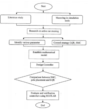
There are certain procedures and methods are used in order to complete the research

and make sure the project is running smoothly. Figure 1.1 shows the flow chart of the

project methodology. The study of the literature review is firstly done, mostly using

the IEEE database as the main source to find the papers and journals regarding to the

related field of this project. The book about the controller including modern strategy

(22)

mathematical model that will be used. The study on the MATLAB/SIMULINK

soft-ware has to be done in order to simulate the final results of the controller system. The

single track mathematical model is used in this research. This mathematical model is

very useful as to represent the dynamic system. After implementing the

mathemati-cal model to the MATLAB/SIMULINK, the simulation of controllable system can be

observed and analyzed. Then the controller is designed to enhance the stability and to

[image:22.595.122.473.241.679.2]

reject the undesired steady state error.

(23)

6

1.6 Thesis Structure

The contents of this thesis are about the flow of the project report. This thesis consists

of five chapters. In the chapter I, the project overview which the objective, scope

of work, problem statement and project methodology are briefly deliberated which

purposely to provide the reader an understanding of the project introduction.

Chapter II, embracing the literature review of the project which includes the

conception, principle, perspective, and the method of the project that is used in

or-der to solve the problem occurs and any assumption that related with the research of

methodology.

Chapter III is about the investigation methodology of the project. This chapter

will discuss the method or approach that used in project development such as

mathe-matical modeling and also includes the software aspect.

Chapter IV discusses briefly on the observation, result and the analysis of the

project that the achievement during the development of project. This chapter also

consists of the final result of the project.

Chapter V covers the discussion of whole contents of the thesis and project

and the recommendation for improvement process in the future research and overall

(24)

CHAPTER 2

LITERATURE REVIEW

2.1 Introduction

The derivations on the modeling of the active car steering systems with linearization

model plant are presented in detail in this chapter. A mathematical derivation is

estab-lished in state space equation of the active car steering. Furthermore, the assumptions

that have been added to the single track car model will be described. In order to

differ-entiate dry and wet road performance, several values of road coefficient, µ are used.

The disturbance profiles which are considered as the disturbance input torque are also

presented in the end of this chapter.

2.2 Background

There are many researches on active safety systems for ground vehicles are having been

up to recent years due to motivated by the ever increasing demand for safety against car

accidents. The active safety systems are included active steering and independent brake

intervention. Active safety systems are developed based on the "by-wire" technologies

to drive the devices independently of the driver’s operation [6]. The by-wire driven

steering and braking systems which are dealt with this article are generated in large

quantities lately [7]. Hence, the by-wire driven active four wheel steering and active

braking system is assumed to be equipped in the vehicles. In order to improve vehicle

lateral stability, the yaw moment is directly controlled by direct yaw moment control

systems by generating differential braking forces between left and right wheels [6].

The lateral tire forces are controlled by the active four wheel steering systems by

gen-erating independent steer angles of front and rear wheels to improve vehicle handling

and stability. Usually, the performance of each control system depends on the status of

(25)

8

By modulating the lateral tire forces, the active steering can regulate the tire slip

angle and affect the vehicle handling behavior. There are three types of active steering

which are Active Front Steering (AFS) [8] [9] [10], Active Rear Steering (ARS) [11]

and Active Four Wheel Steering (W4S) [12]. By using disturbance observer control

method [8] [13], sliding mode control [14], predictive control [9], or other control

tech-niques, this latter may be established. By applying an additional steering angle to the

driver’s steer command, normally the active handling control will serve a steering

sup-port system. The AFS potential is usable once Steer-by-wire technology is established

because of the extra steering action.

The lateral acceleration of the front axle may be robustly triangularly decoupled

from the yaw rate dynamics [15]. This is because it is using only the front wheel

steering angle as a control input which is feeding back the yaw rate error through an

integrator. For braked and unbraked driving condition, a PI active steering control on

the yaw rate tracking error with different gains is used [16]. In order to ensure safety

also during a system failures,the active front steering is designed [17]. The wheel

steering angle,δf is the sum of the designed feedback control,δcand the driver input,

δp[18].

The development of electro actuated differentials allows for new control

strate-gies in vehicle systems dynamics control [19] [20]. The differential control system is

semi-active which the electronic control system can decide the locking torque

trans-ferred but not its direction [19]. While the transfered torque is generated from the

fastest wheel to the slowest one and the control operates when the rear wheels speed

difference exceeds a given threshold. A proportional-integral control law computes

the value on the measured and the desired rear wheel speed angular velocity. The

pro-posed controller is designed following the Internal Model Control approach and since

it can generate yaw moments of every amount and direction thus it is activated [20].

According to a Lyapunov analysis, it is electronically controlling the locking action of

the rear differential [18] [21].

An integrated control of active front steering and direct yaw moment which

(26)

program (ESP) is integrated with the active front wheel steering, active suspension and

active anti roll bar [23]. Four wheel steering are coordinated with wheel torque

dis-tribution by using an optimization approach is shown [24]. A non linear optimization

is approached to determine the optimal force to be exerted by each tire controlled by

active steering and brake pressures distribution [18] [25].

Active front steering is a newly developed mechatronic steering system for

pas-senger cars that realizes an electronically controlled superposition of an angle to the

hand steering wheel angle that is prescribed by the driver, cf [26].

A steering aid system integrated in cars is known as Active Steering. There

are many different systems with different control strategies on the market. The main

purpose is to improve safety and comfort of the vehicles by improving the stability and

handling of the steering. The actuators are still used to influence the mechanical system

even though the regulations demand a mechanical connection between the steering

wheel and the steering rack.

Active steering is an effective way that can improve drivers comfort and

han-dling. The vehicle handling and lateral stability can be controlled at the same time, if

both the external yaw moment and active steering angle are adopted [27].

Active steering can be said as an integrated steering support system for cars.

The system is like the steering on conventional cars but with additional functionality

which can withstand with disturbances. For example,µ-split which is a split adhesion

coefficient between wheels, wind gusts or decreased road adhesion conditions. There

are various types of systems are conceptual and not intended for the market. However,

BMW has a semi-mechanical system installed on the five hundred and thirty cars.

The main purpose for changing the steering characteristics of a car is to improve

safety and comfort of the vehicle. The following sections will describe a specific

(27)

10

2.3 Research of Active Front Steering System

The steering system can be said is an important role of making car convenient to handle

and enhance the vehicle stability. The steering system development has experienced

many stages,and the newest technology of steering system for passenger cars is the

Steer-by-Wire system (SBW). However, the Steer-by-Wire system is permitted by state

regulations because of it has not yet accepted by public consumers in the

considera-tion of the reliability and safety of the system. A newly technology for passenger cars

which is developed by BMW is Active Front Steering (AFS). This technology is

im-plementing an electronically controlled superposition of an angle to the hand steering

wheel angle which is prescribed by the driver. However, the connection of permanent

mechanical between steering wheel and road wheels are remained [1]. The vehicle

performance can be adjusted by AFS through intervening the road wheel angle in

con-dition of the driver have top priority.

For the active steering system, the variable steering gear ratio function will be

experienced by the driver first. Then perceive the improvement of steering portability

[1]. According to the vehicle’s motion state, AFS enables continuous and

situation-dependent variation of the steering ratio. Therefore, the maneuverability of the vehicle

at low speed and the stability at high speed are improved by the AFS. The performances

of the improvement of the stability with active steering system depend on the variation

quality of the steering ratio to a certain extent. Thus, the variable steering gear ratio

function is important to be investigated.

Active steering system is comprised of a double planetary gear and an electric

actuator motor additionally which is compared with traditional mechanical steering

system [1]. The AFS is reliable and safe due to all the links from the steering wheel to

road wheel are mechanical. AFS can ensure that the vehicle is under driver’s control

and make driver have a clear road feel. From the Figure 2.1 below shows that the

AFS’s planetary gear have two degrees of freedom (DOF), the planetary gear output

connects with the steering gear’s pinion and one input connects with the steering wheel

(28)

[image:28.595.119.543.74.204.2]

Figure 2.1: (a) Schematic view of AFS system; (b) 3D-model of planetary gear set and electric motor [1].

2.4 Vehicle Dynamics Modeling

According to the SAE standard which is described in SAE J670e, the vehicle axis

system used throughout the simulation [28]. First, the derivation of that model which

includes the tire model is discussed. The motion equations are converted into a state

space form for easily to do integration and a Third Order Runge-Kutta integration is

used as the integration algorithm. Lastly, in order to show its validity, the vehicle

model is verified against results from Smith et al. [2].

2.4.1 Vehicle Axis System

According to SAE J670e [28] as shown in Figure 2.2 below, the coordinate system is

used in vehicle dynamics modeling. The x-axis which is referred to the forward

direc-tion or the longitudinal direcdirec-tion. while the y-axis is referred to the lateral direcdirec-tion

which is positive when it points to the right of the driver. And lastly, the z-axis is

represented to the ground satisfying the right hand rule.

Only the X-Y plane of the vehicle is considered which among most studies

(29)

[image:29.595.157.486.71.232.2]

12

Figure 2.2: Vehicle Axis System after SAE [2].

used in the study of ride, pitch, and roll stability type problems [2]. The relevant

definitions for the variables associated with this research are defined in the following

list.

Longitudinal direction which is a forward moving direction of the vehicle.

There are two different types of methods to look at the forward direction. One of

them is with respect to the vehicle body itself and the another is with respect to a fixed

reference point. When dealing with acceleration and velocity of the vehicle, the

for-mer is often used. The latter is used during the location information of the vehicle with

respect to a starting point or an ending point is desired [2].

While the lateral direction is a sideways moving direction of the vehicle. Same

as the longitudinal direction, the lateral direction also has two ways of looking which

are with respect to the vehicle and with respect to a fixed reference point. The

ex-treme values of lateral acceleration or lateral velocity can decrease the stability and

controllability of vehicle.

The tire slip angle is equivalent to heading in a given direction but walking at

an angle to that direction by displacing each foot laterally. Because of the presence of

lateral forces the foot is displaced laterally.

Lastly, the body-slip angle is the angle between the X-axis and the velocity

vector that represents the instantaneous vehicle velocity at that point along the path

(30)

Although the concept is same, but each tire may have different slip angle at the same

time. Sometimes the body slip angle is calculated as the ratio of lateral velocity to

[image:30.595.158.486.157.383.2]

longitudinal velocity [2].

Figure 2.3: Vehicle Axis System after SAE [2].

2.4.2 Vehicle Models

There are many types of degrees of freedom (DOF) which are associated with

vehi-cle dynamics. A two-degree-of-freedom bicyvehi-cle model is the most simplified vehivehi-cle

dynamic model which is representing the lateral and yaw motions. The idea for this

model is that sometimes the longitudinal direction is not necessary or desirable to be

included due to the lateral or yaw stability of the vehicle does not be affected by the

longitudinal direction. Usually this model is used in teaching purposes. Figure 2.4

(31)

[image:31.595.193.449.75.183.2]

14

Figure 2.4: Two Degree of Freedom Model [2].

While for a three-degree-of-freedom model, it adds longitudinal acceleration to

the model. Thus, it enables one to describe the full vehicle motion in the X-Y plane.

The longitudinal velocity, U, and the longitudinal force,F_{t f} andFtr, are included into

the model which is shown in the Figure 2.5. This is the model that is used in this

project [2].

Figure 2.5: Three Degree of Freedom Model after Smith [2].

Lastly, the symmetry in dynamic behavior between right and left sides is no

longer assumed for an eight-degree-of-freedom model. Instead of two tires, the

rota-tional degree of freedom for each of the four tires is considered in this vehicle model.

A rolling motion,φs is added between left and right sides of the vehicle. This model

is frequently used in the suspension design or ride comfort analysis, especially for the

[image:31.595.165.479.367.470.2]

(32)

[image:32.595.171.473.79.301.2]

Figure 2.6: Eight Degree of Freedom Model after Smith [2].

2.5 Car Modeling

From the Figure 2.7 below shows that the car is modeled as a rigid body with mass

mand moment of inertiaJ with respect to a vertical axis through the center of gravity

(CG). The yaw angle ψ rotates the chassis coordinate system x,ywith respect to an

inertially fixed coordinate systemx₀,y₀. The yaw rate is r=ψ which is measured by

a yaw rate sensor. The yaw rate will be used as one of the state variables in the state

vectorx[29].

[image:32.595.182.462.521.704.2]

(33)

16

The most significant uncertainties for modeling the motion of this vehicle are

the lateral forcesF_yR which is at the rear axle andF_yF which is at the front axle. The

lateral forces and rear axle are depended on the state x of the car. The front lateral

force depends on the front wheel steering angleδF. In the automotive literature there

are tire models that give the lateral forces. Yet, the forces are described in terms of

other quantities, such as the road friction coefficient µ. Therefore, the forcesFyR and

FyF directly as the uncertain quantities.

A position at a distance l_p in front of the CG is needed to be chosen as the

lateral accelerationayPat this point does not depend onFyR. It is a calculation of a few

lines to find the position and the calculation is shown in (2.1).

l_p= J

ml_R (2.1)

Thus, the lateral acceleration is

a_yP= l

ml_RFyF(x,δF) (2.2)

wherel=l_R+l_F is the wheelbase which can be seen at Figure 2.7

2.5.1 Mathematical Modeling For a Single Track Model

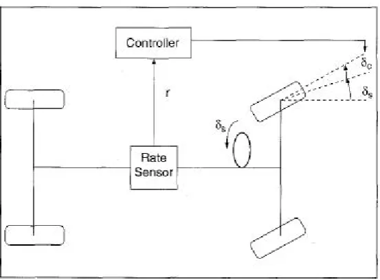
In the Figure 2.8, it shows the implementation of a steering control system. The driver

is handling the main steering angle, δS from the steering wheel. An actuator sets a

small corrective steering angle with input from a feedback controller. The yaw rate

and the superpositionδF =δS+δCis the main feedback signal which can be arranged

mechanically. The tire forces are depended on the state variables of the chassis and

(34)

[image:34.595.182.459.72.276.2]

Figure 2.8: The steering angleδF =δS+δCis composed of the commandδS, from the

driver and the feedback controlled additional angleδC.

A single track car model is used to describe the dynamics of vehicle steering.

By combining the two front wheels into one wheel which refers the center line of the

car, same as the two rear wheels, the single track model is obtained. Thus, in Figure

2.9 below shows the car model is reduced which describes the yaw rate and lateral

motions.

[image:34.595.154.494.523.691.2]

(35)

18

The anglesδF andδR are referred to the front and rear steering angles

respec-tively. The distance between the center of gravity (CG) and the front axle is represented

aslF and rear axle is represented aslR. Thus, the wheelbase is referred to the sum of

the front axle and rear axle,l=l_R+l_F. The vehicle sideslip angle which is the angleβ

is the angle between the vehicle center line and the velocity vectorvat the CG. In the

horizontal plane which is shown in Figure 2.9 shows that an initially fixed coordinates

system(x0,y0)is together with a vehicle fixed coordinates system(x,y)that is rotated

by a yaw angleψ. In the dynamic equations, the yaw rater:=ψ will appear as a state

variable.

The model of automatic car steering will include the yaw angle ψ where the

position of the vehicle relative to the lane is considered. The forces which are the side

forcesF_ytF andF_ytR that are transmitted between the road surface and the car chassis

through the wheels are shown in Figure 2.9. The forces in the longitudinal direction of

[image:35.595.160.480.416.549.2]

the tires are assumed to be zero for example the wheels are freely spinning.

Figure 2.10: Lateral forcesF_ytFat the front wheel in tire coordinates andF_yF in chassis

coordinates.

The velocity vector vF which under a sideslip angleβF at the front axle with

respect to the longitudinal axis (x-axis) of the chassis is represented in Figure 2.10. A

function of the tire slip angleαF =δF−βF is known as the lateral forceFytF in tire

coordinates. The dominants component in chassis coordinates is shown in equation

(36)

F_yF =F_ytFcosδF (2.3)

If it occurs symmetrically at the left and right wheel, the small retarding

com-ponentFxF =−FytFsinδF does not generate a yaw torque. The longitudinal effect is

compensated by speed control. The speed control is automatic or controlled by the

driver. In a static tire description, the tire side forces FytF is a function of the tire slip

angleαF.

F_ytF= f(αF) = f(δF−βF), (2.4)

F_yF = f(δF−βF)cosδF (2.5)

The front wheels are indicated by the index F which it is replaced by R for the

rear wheels. The lateral force is zero, f(0) =0 if the velocity vectorvF is aligned with

the tire. The lateral force is close to saturate for αA >10. A control system cannot

overcome on the physical limits. Thus, design steering controllers is very important

for that only small tire sideslip angles occur.

The lateral forces at the front and rear axles are the inputs to the vehicle dynamics

which shown in equation below:

F_yF =F_ytFcosδF

F_yR=F_ytRcosδR

(2.6)

While for longitudinal force component:

(37)

20

These forces represents the sum of the forces at the left and right tire. Through

the dynamics model, the forces control state variables are β, v and r. The motions

equations for 3-Degree-of-Freedom in horizontal plane

are:-1. Lateral motion

mv(β+ψ)cosβ+mvsinβ =FyF+FyR (2.8)

2. Longitudinal motion

−mv(β+ψ)sinβ+mvcosβ =Fx (2.9) 3. Yaw motion

Jψ=FyFlF−FyRlR+MzD (2.10)

It is obtained from equations (2.8) to (2.10) withr:=ψ.



   

mv(β+r)

mv Jr      =     

-sinβcosβ0

cosβsinβ0

001           F_x F_yF+F_yR F_yFl_F−F_yRl_R+M_zD

     (2.11)

From the kinematic model which denotes the steering angles δF,δR and the

state variables β,randv, the sideslip anglesαF andαR at the front and rear tires are

obtained. TheβF andβR are the front and rear chassis sideslip angles. The velocity

components in the longitudinal direction of center line of the vehicle is equal

(38)

The yaw rate, r will affect the relationship between the velocity components and the center line, as it is shown as below:

vFsinβF =vsinβ+lFr

vRsinβR=vsinβ+lRr

(2.13)

By the corresponding terms from equation (2.12), the velocity terms v_F and v_R are

eliminated by division. So that, the kinematic model is

tanβF =

vsinβ+lFr

vcosβ =tanβ+

lFr

vcosβ

tanβR=

vsinβ+lRr

vcosβ =tanβ+

lRr

vcosβ

(2.14)

In Figure 2.10, it shows that the tire sideslip angles are

αF =δF−βF

αR=δR−βR (2.15)

By the non-linear tire model, the feedback-structured model is completed:

F_ytF= f_F(αF)

F_ytR= f_R(αR)

(39)

22

2.5.2 Linearization for Constant Velocity and Small Angles

The vehicle dynamics which is shown in equation (2.11) are nonlinear. By taking the

assumptionv=0, these equations can be linearized. It can be justified because of the

velocity, v is changing more slowly than the state variables r and β. The velocity, v

is now treated as an uncertain constant parameter. In addition, the force component

F_xsinβ is neglected. Next, the linearized version of equation (2.11)

is:-

 ˙

mv(β+r) ˙ Jr  =  

(F_yF+F_yR)cosβ

F_yFl_F−F_yRl_R+M_zD



 (2.17)

Due to the chassis sideslip angles such asβ,βF andβR are small, thus cosβ =1 and

becomes:-βF =β+lFr/v

βR=β+lRr/v

(2.18)

Then, the steering angles such as δF,δR are small as well, for the rear wheels the

cosδF =1 and cosδR=1. Thus,

F_yF =F_yF(αF)

F_yR=F_yR(αR)

(2.19)

The equations above are the unknown characteristics. Hence, the equation (2.17) will

become:-

 ˙

mv(β+r) ˙ Jr  =  

FyF(αF) +FyR(αR)

F_yFl_F−F_yRl_R+M_zD



 (2.20)

(40)

From the Figure 2.8 for the feedback control , the steering anglesδF is the sum

of the driver commandδswith the corrective angleδcwhich both of them are generated

by the feedback system. The relationship betweenδs,δcandαF,βF are demonstrated

by Figure 2.10.

The lateral tire forces are now linearized about a zero tire sideslip angle as in

equation (2.16) in order to allow for a linear analysis of the car.

FyF(αF) =µcF(αF)

FyR(αR) =µcR(αR)

(2.21)

The cornering stiffness is the slope c_F and c_R of the tire characteristic. The

friction coefficient µ <=1 is assumed that both the front and rear wheels are same.

The representative values of the friction coefficientµ are:

µ =1(dryroad)

µ =0.5(wetroad)

µ =0.15(icyroad)

Thus, equation (2.20) is interpreted forβ andrby substituting the linearized tire

char-acteristicsFyF andFyR:

  ˙ β ˙ r  =   µ

mv(cFαF+cRαR)−r

µ

J(cFlFαF+cRlRαR) + 1 JMzD



 (2.22)

Development Of Active Steering Control Based On Sliding Mode Control With The Inclusion Of An Observer